

What the module calculates
Point load gives the stress increase in the ground below one or several vertical point loads on the ground surface, by Boussinesq’s solution for a homogeneous, elastic, isotropic half-space. You place the loads on the surface, choose a point A inside the soil, and the module gives the vertical stress increase Δσz and the horizontal stress increases Δσx and Δσy there, the lines of equal stress, the colour contours, the stresses under A against depth and a 3D view.
For one load the stresses depend on the horizontal distance r of the point from the load and on its depth z; L is the distance of the point from the load:
In the horizontal formula x and y are the distances of the point from the load, x − xL and y − yL; Δσy is the same with x and y exchanged. With μ = 0.5 the second terms vanish. Δσz does not depend on Poisson’s ratio μ; the horizontal stresses do. Several loads each act alone on the half-space and their stresses add.
What you can describe
- One to eight vertical point loads on the ground surface, each with its force P and its position (xL, yL); no two loads may stand at the same place.
- A point A below the surface: its position x, y on the ground and its depth z.
- Poisson’s ratio μ of the soil, for the horizontal stresses only.
- The depth of the profile zmax: how far down the profile of the stresses under A is drawn.
The module gives the three stress increases at A (and, for one load, the influence factor I1, r and L), the working step by step, the stresses under A at ten depths and at A itself, and a report as a PDF or Word file. The stresses are the increases caused by the loads; they add to the stresses already in the ground.
Which module for which load
- A load spread along a line, over a strip, a rectangle or a circle, or an embankment: use the other modules of the family, for example Vertical line load, Vertical strip load, Rectangle, Circle, any point and Embankment. The family page lists all twelve.
- A loaded area of any shape: Influence chart.
- Layered ground, with Westergaard’s solutions: Westergaard point load and Westergaard areas.
- The pressure of a surcharge on a wall: the Surcharge loads manuals.
Before you start: what you need
Have these ready from your design:
| What | Notes |
|---|---|
| What From: where it comes from | Notes |
| The loads P From: your design | Each is a vertical force on the ground surface: zero or more. Up to eight. |
| The position of each load From: your layout | The coordinates xL and yL on the ground surface. The first load may stand at the origin. |
| The point A From: the place you want the stress | Its position x, y on the ground surface, in the same coordinates as the loads, and its depth z below the surface (at least 0.001 m). |
| Poisson’s ratio μ From: your soil data | From 0 to 0.5; 0.5 for an undrained clay. It changes the horizontal stresses only. |
| The depth of the profile zmax From: the depth you want to see | At least 0.1 m. |
Quick start in seven steps
- Open the module and choose the units
Open Point load from the Stresses in a Soil Mass family. Pick SI · kN, SI · tf or US in the header; you can change it at any time.
- Enter the load
In Point loads the first load is already in the table. Press its row to change P, xL and yL. To add more, fill the New point load form and press + Add point load.
- Place the point A
In Point of interest type x, y and the depth z, or drag the blue dot A on the Section drawing.
- Set Poisson’s ratio and the profile depth
In Soil type μ (0.5 for an undrained clay). In Depth profile type zmax, or drag the dashed line at the bottom of the Section.
- Press Analyze
Press Analyze at the foot of the Model tab. The bar reads Analysed — the stresses at the point calculated, the loads lock, and the lines of equal stress appear on the Section (in the Section view).
- Read the answer
The Results tab gives Δσz, Δσx and Δσy at A. Drag A on the Section or the Contours to read the stress elsewhere; the answer follows at once.
- Take the working and the report
The Calculations tab writes out the steps with your numbers. The Report tab saves a PDF or a Word file.
The screen: section, contours, profile and 3D
The layout is the one every GeoTerva module shares, described in the workspace guide. The drawing has four views, chosen with the buttons above it:
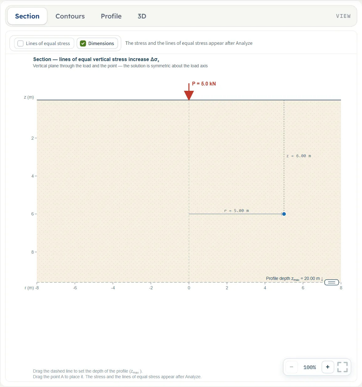
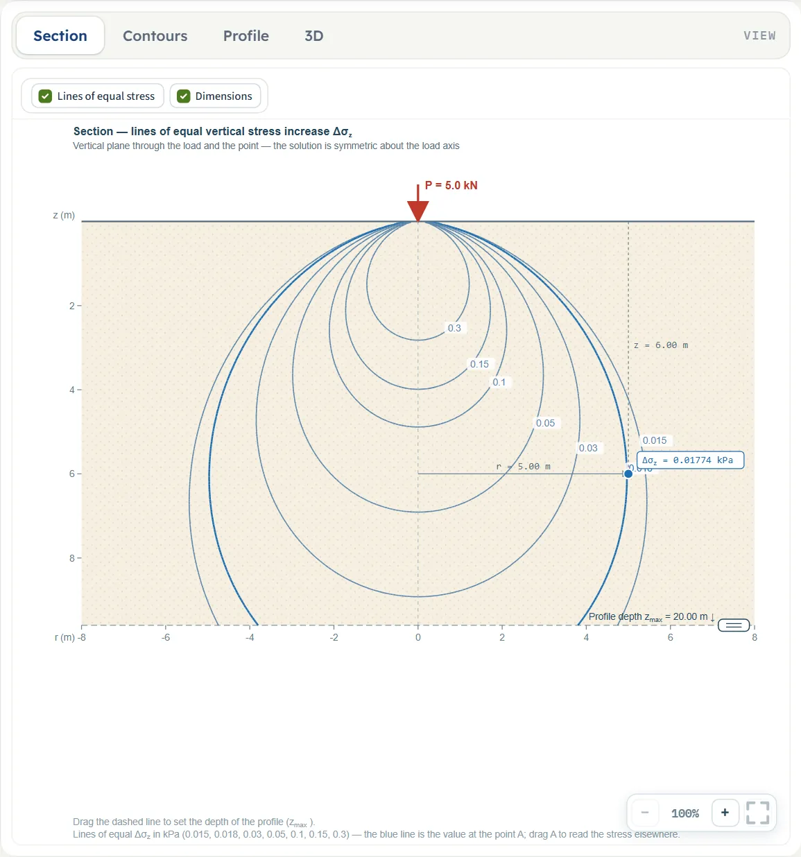
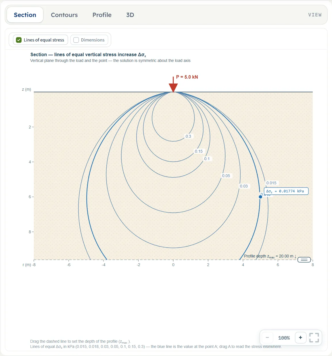
- Section is a vertical cut through the ground. With one load it is the plane through the load and the point A, and the solution is symmetric about the load axis, so the horizontal axis is the distance r from the load. With several loads it is the vertical plane y = y through A, parallel to x, and the loads that stand beside the plane are marked “beside the plane”: they act on it as well. After Analyze it carries the lines of equal vertical stress increase and the value at A.
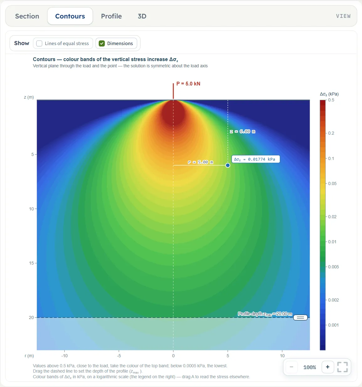
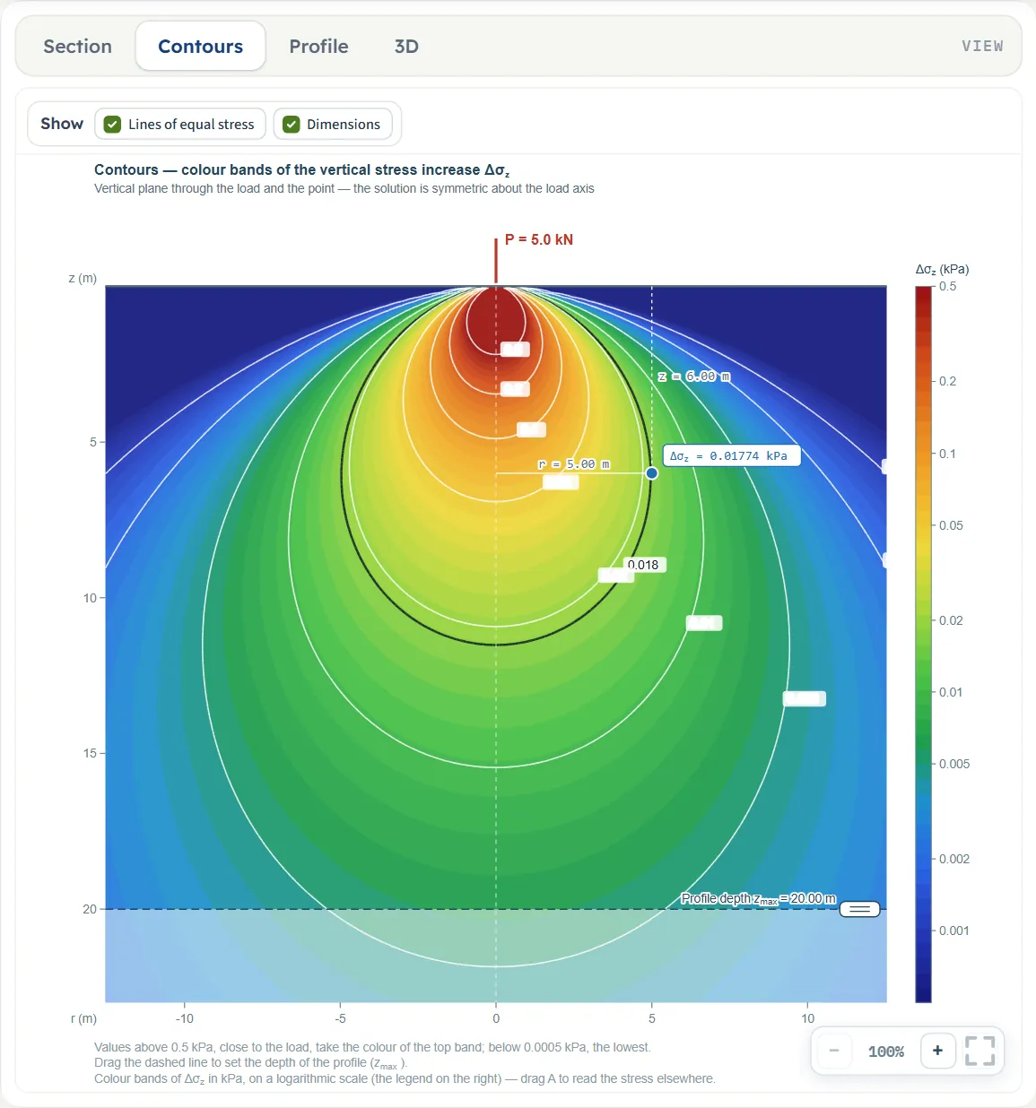
- Contours is the same cut with the vertical stress increase in colour bands on a logarithmic scale, with the legend on the right. Values above the top of the scale take the colour of the top band; values below the bottom, the lowest.
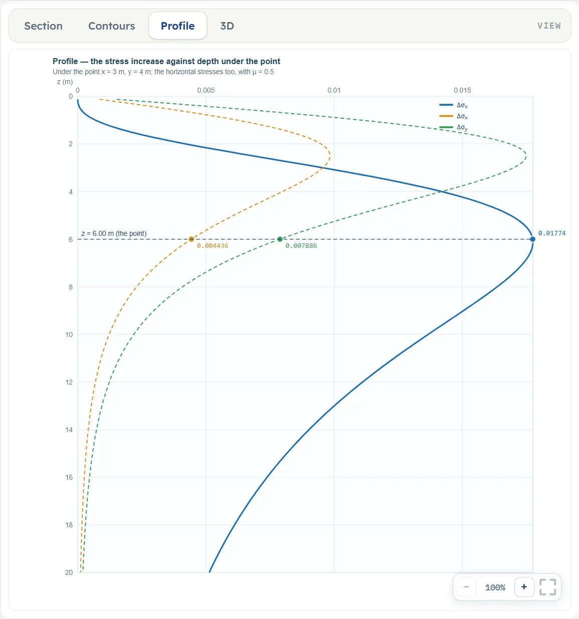
- Profile is the stress increase against depth under A: Δσz as a solid line, Δσx and Δσy dashed, with the values at the depth of A.
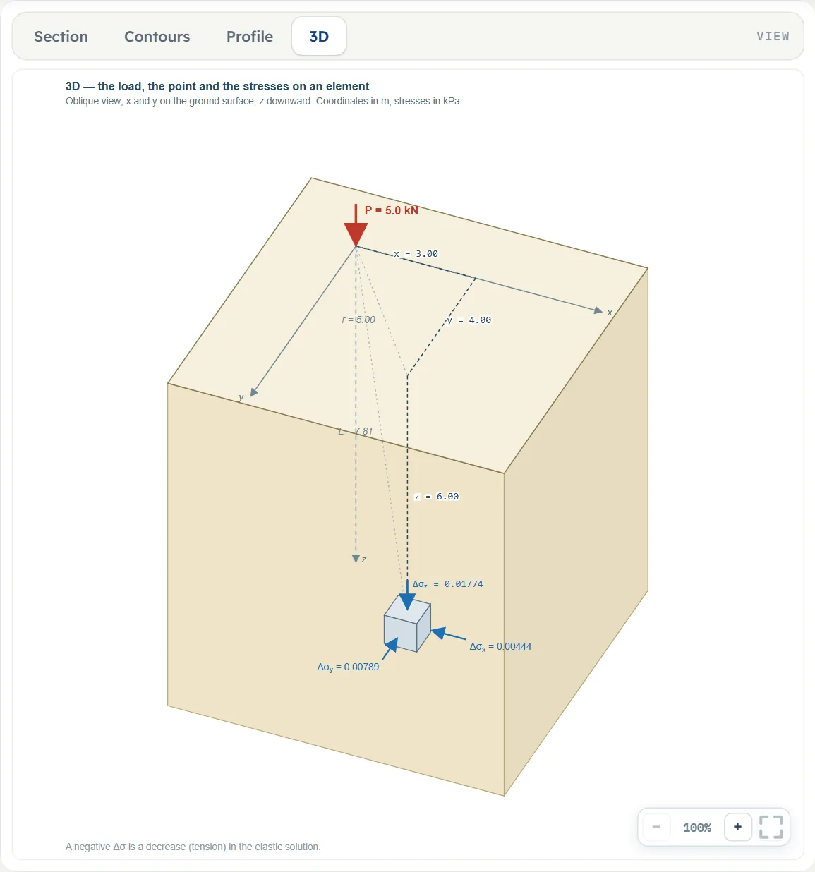
- 3D is an oblique view of a block of ground with the loads, the distances x, y, z and an element at A with the three stresses on it.
The Show chips
Above the Section and the Contours a bar holds two chips (on the Contours it is headed Show). Lines of equal stress draws the lines of equal vertical stress; on the Section it is checked once the model is analysed, on the Contours it starts unchecked. Dimensions draws the dimension lines of the distance r (or x − xL) and of the depth z of A, and is on by default; the label with the value at A stays when it is off. Before Analyze the lines chip is unchecked and cannot be switched on; the Section bar says “The stress and the lines of equal stress appear after Analyze” and the Contours bar says “The colour contours of the stress appear after Analyze”. The Profile and the 3D views have no chips.
What you can drag
- The point A on the Section and the Contours, before and after Analyze. With one load a horizontal pull moves A along the direction from the load (x and y change together, so r changes) and a vertical pull changes z. With several loads a horizontal pull changes x and y stays. With one load the distance r and the depth z move in steps of 5 cm and x and y follow, rounded to 0.01; with several loads x and z move in steps of 5 cm. A stays inside the frame of the drawing; the boxes of the Point of interest section follow. After Analyze the answer is recalculated at once for the new place.
- The dashed line at the bottom of the Section and the Contours sets the depth of the profile zmax (at least 0.1 m), before and after Analyze.
- A load, before Analyze only. In the 3D view the arrow of a load is pulled over the ground, so xL and yL change together; when there are several loads, the arrows on the Section and on the Contours are pulled along x as well. All move in steps of 5 cm. A load cannot be pulled onto another one: it stops at the last free place and the module says “Another point load already stands at this position — the value is kept as it was.” With one load the Section has no handle on the load; use the 3D view or the boxes.
- Nothing else: the value of Poisson’s ratio and the loads are typed, and after Analyze the loads and μ are locked until you press Edit inputs, which also clears the results.
Zoom
Each view has −, a percentage and + at the lower right, and a button that fits the whole drawing in the pane. The mouse wheel zooms as well, and a zoomed drawing is moved by dragging its background.
Entering the model, section by section
The Model tab has five sections: Model data, Point loads, Point of interest, Soil and Depth profile. Each opens when you click its title; Next and Back at the foot walk you through them, and Analyze waits below the last one. In the tables, a unit shown three times, such as kN · tf · kip, gives the units of SI · kN, SI · tf and US in turn; equal ones are merged. Defaults are shown in SI; in US the boxes show the converted values, for example 9.84252 ft for x = 3 m.
Model data
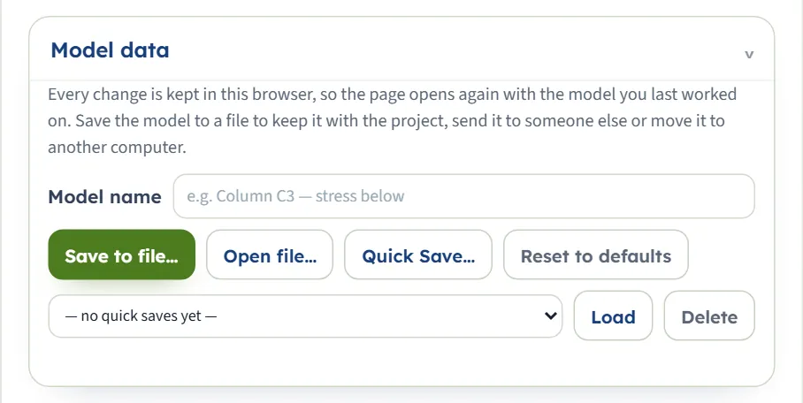
The first section holds the model name, Save to file…, Open file…, Quick Save… with its list and Load and Delete, and Reset to defaults. It works as described in the workspace guide. Reset returns the example at once and the page keeps it as the model of the browser.
Point loads
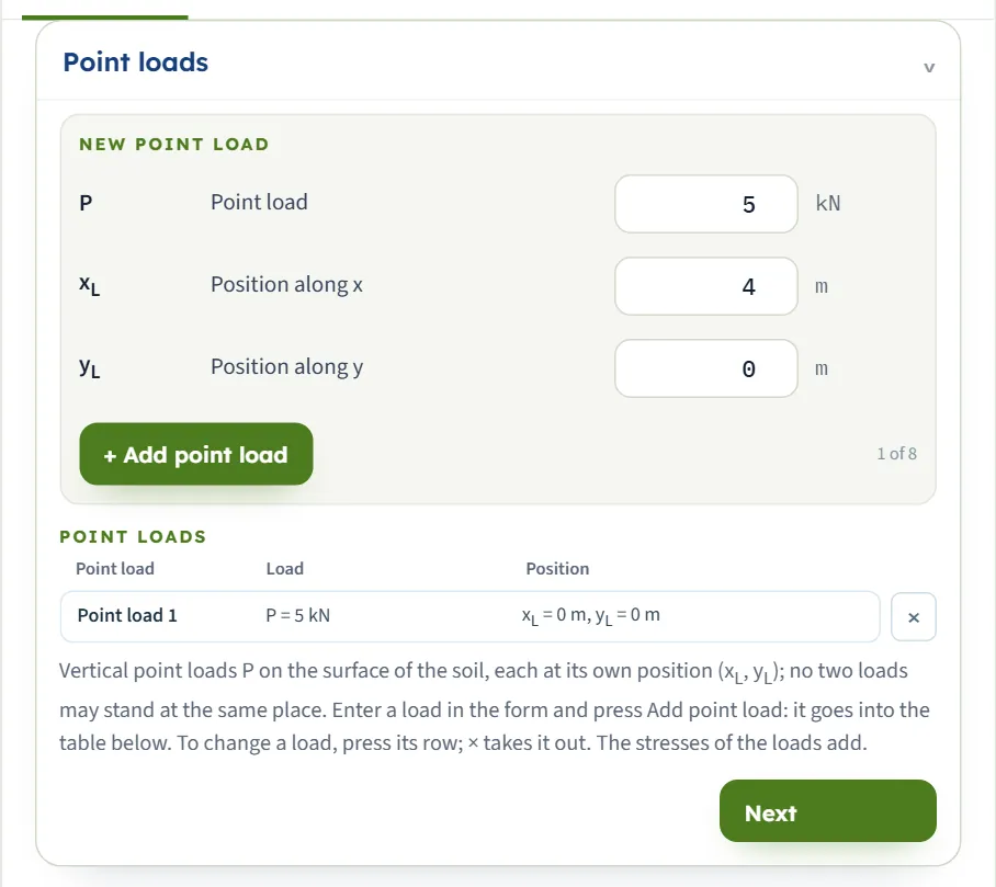
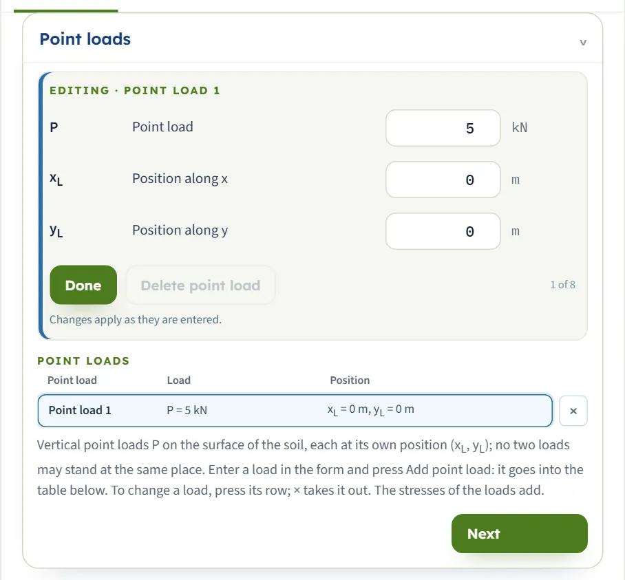
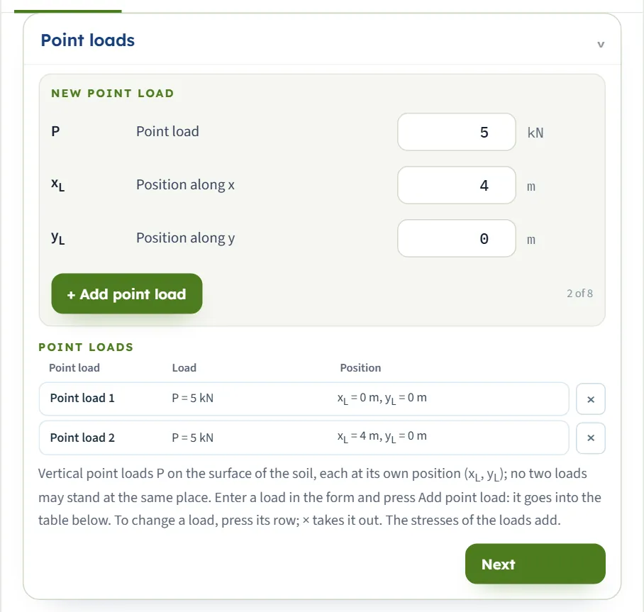
The section is a form over a table. The New point load form takes P, xL and yL of one load; + Add point load puts it into the table, and a counter beside the button shows how many of the eight loads there are. On a fresh page the form opens with P = 5, xL = 4 and yL = 0 (the first load of the model stands at the origin); after you add a load it keeps the values you entered. Press a row of the table to change that load in the form (the form then reads Editing · Point load 1 and offers Done and Delete point load; changes apply as they are entered), or press × to take a load out (it is disabled while only one load remains). With eight loads the add button is disabled.
| Field | Unit | Default |
|---|---|---|
| Point load P The vertical force on the ground surface. Zero or more. | kN · tf · kip | 5 |
| Position along x xL The place of the load on the ground surface. The form starts with 4. | m · ft | 0 |
| Position along y yL The place of the load on the ground surface. | m · ft | 0 |
Point of interest
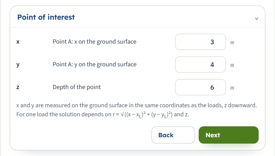
The three coordinates of the point A. The note under the fields says that x and y are measured on the ground surface in the same coordinates as the loads, with z downward, and that for one load the solution depends on r and z. Typing the numbers and dragging A on the drawing do the same thing.
| Field | Unit | Default |
|---|---|---|
| Point A: x on the ground surface x In the same coordinates as the loads. | m · ft | 3 |
| Point A: y on the ground surface y In the same coordinates as the loads. | m · ft | 4 |
| Depth of the point z Measured down from the ground surface. At least 0.001 m. | m · ft | 6 |
Soil
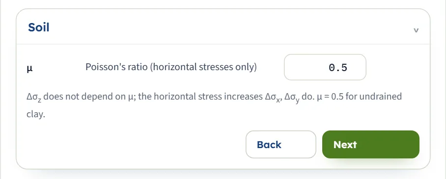
One number. The note says that Δσz does not depend on μ, that the horizontal stress increases do, and that μ = 0.5 is for an undrained clay.
| Field | Unit | Default |
|---|---|---|
| Poisson’s ratio (horizontal stresses only) μ From 0 to 0.5. It does not change Δσz. | — | 0.5 |
Depth profile
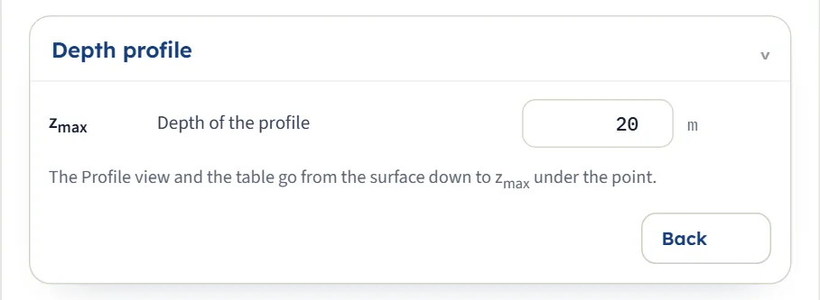
One number again: how far down the profile under A is drawn and tabulated. A depth smaller than the depth of A is accepted: the table then ends at the depth of A and the Profile view a little below it, while the dashed line stays at the depth you typed.
| Field | Unit | Default |
|---|---|---|
| Depth of the profile zmax At least 0.1 m. The Profile view and the table go from the surface down to this depth under A; if it is smaller than the depth of A, the table ends at the depth of A and the Profile view a little below it. | m · ft | 20 |
Choosing the loads, the point and Poisson’s ratio
The module has no method to choose: the solution is Boussinesq’s. What you decide is where the loads and the point stand, and μ.
| Choice | What it does |
|---|---|
| Number of loads | Each load acts alone on the half-space and the stresses add. One load gives the symmetric section about its axis, with I1, r and L on the Results tab; several loads give the stresses of their sum, and the Calculations tab shows each load and then the total. |
| Position of A | On the axis of a load (x = xL, y = yL) the vertical stress is largest for that depth: at 6 m, I1 = 0.4775 and Δσz = 0.06631 kPa for 5 kN, against 0.01774 kPa at 5 m to the side. |
| Poisson’s ratio μ | Changes Δσx and Δσy; Δσz stays the same. Use 0.5 for an undrained clay. Under the load axis the two horizontal stresses are equal and, for μ below 0.5, negative: a decrease. |
Which should I pick?
- Several loads when the loads are distinct and the ground between them is the same: add each, with its own force and position. For a load spread over an area use a module of that shape.
- The point where the design needs it: the centre of a layer for a settlement calculation, or the level of a buried structure. Drag A to read the stress elsewhere and compare it with the profile.
- μ = 0.5 for an undrained clay; for a drained soil, use the value from your soil data. The vertical stress, which settlement calculations use, does not depend on it.
Analyze and read the results
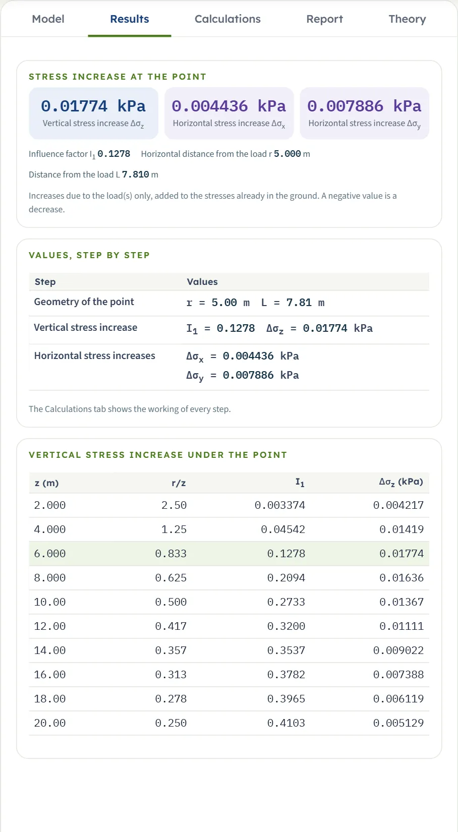
Press Analyze. The bar changes to Analysed — the stresses at the point calculated and says “The inputs are locked. Edit inputs clears the results; the unit system can still be changed. The point A stays free: drag it on the drawing or change its coordinates, and the stress there is calculated at once.” The page may stay on the Model tab: open the Results tab for the answer.
| Card | Symbol | The example |
|---|---|---|
| Vertical stress increase | Δσz | 0.01774 kPa |
| Horizontal stress increase | Δσx | 0.004436 kPa |
| Horizontal stress increase | Δσy | 0.007886 kPa |
| Influence factor (one load only) | I1 | 0.1278 |
| Horizontal distance from the load (one load only) | r | 5.000 m |
| Distance from the load (one load only) | L | 7.810 m |
Below the cards, Values, step by step lists r, L, I1 and the three stresses, and a table gives the stresses under A at ten equal depths down to zmax (or down to the depth of A, if that is deeper) and at A itself, whose row is highlighted. For one load the table has the columns z, r/z, I1 and Δσz; for several loads it has z, Δσz, Δσx and Δσy. A line under the cards says: “Increases due to the load(s) only, added to the stresses already in the ground. A negative value is a decrease.”
Using the numbers
- The stresses are increases. Add them to the stresses already in the ground (the effective stress from the weight of the soil) before you use them.
- The stress is in kPa, t/m² or ksf, by the unit system. The same example gives 0.001809 t/m² and 0.0003706 ksf.
- A load of zero is accepted and gives zero stress; the loads add, so a load that stands directly above A adds to Δσz and adds nothing to the horizontal stresses when μ = 0.5.
- Changing the unit system after Analyze re-states the cards without a new run. Edit inputs unlocks the loads and clears the results.
Warnings and notes
The bar carries a Warnings (0) button. It opens a window that says “No warnings — the assumptions of the solution hold for these inputs.” A condition that stops the analysis is shown as a message, see Messages.
The Calculations tab, the report and the Theory tab
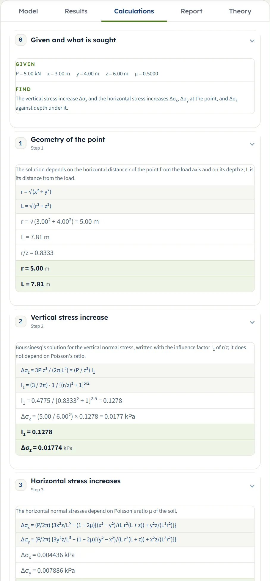
The Calculations tab opens with Given and what is sought and then writes out the working in numbered steps, ending with the answer. For one load:
- Geometry of the point — r = √(x² + y²) (or with x − xL and y − yL when the load is off the origin), L = √(r² + z²) and r/z.
- Vertical stress increase — Δσz = 3P z³ / (2π L⁵) = (P / z²) I1, the value of I1 and the result.
- Horizontal stress increases — the two formulas with μ, the values, and with μ = 0.5 the shorter form.
- Stress increase against depth — the same equation down the vertical line through A, as a table.
For several loads, step 1 is Stress of each load (r, L, I1 and Δσz of every load), step 2 is Superposition (Δσz = Σ Δσz of the loads, written as the sum of the numbers) and steps 3 and 4 give the horizontal stresses and the depth table of the sum.
The report
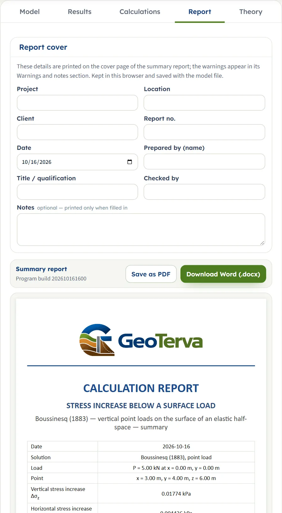
In the Report tab fill in the cover (project, location, client, report number, date, prepared by, title or qualification, checked by, and optional notes). The details are kept in this browser and saved with the model file. Save as PDF and Download Word (.docx) produce the summary report; the preview below the buttons is the report itself.
The report has six parts: 1 Introduction and scope, 2 Input data (a table of the loads and the point, with the section, the profile and the 3D drawings), 3 Calculation (the steps of the Calculations tab), 4 Results, 5 Summary and 6 References. It states the units used.
The Theory tab
The Theory tab has six sections: Scope and assumptions, Boussinesq’s solution, The influence factor I1, Lines of equal stress, Worked examples and References. Each opens when you click its title; Open all and Close all open or close them together. The figures and tables in it are computed from the equations.
Worked example: the module’s own example
The module opens on this example, so you can follow the numbers on your own screen.
| Section | Input | Value |
|---|---|---|
| Point loads | Point load 1 | P = 5 kN at xL = 0, yL = 0 |
| Point of interest | Point A | x = 3 m, y = 4 m, z = 6 m |
| Soil | Poisson’s ratio | μ = 0.5 |
| Depth profile | Depth | zmax = 20 m |
Step 1: the geometry
r = √(3² + 4²) = 5.00 m, L = √(5.00² + 6²) = 7.81 m and r/z = 5/6 = 0.8333.
Step 2: the vertical stress
Step 3: the horizontal stresses
With μ = 0.5 the formulas reduce to Δσx = 3P x²z / (2π L⁵) = 3 × 5 × 9 × 6 / (2π × 7.810⁵) = 0.004436 kPa and Δσy = 3P y²z / (2π L⁵) = 0.007886 kPa, the ratio of the two being 4²/3². These are the three cards of the Results tab and the steps of the Calculations tab.
On the load axis
Move A to x = 0, y = 0 (still at 6 m): r = 0, I1 = 3/(2π) = 0.4775 and Δσz = 0.4775 × 5/36 = 0.06631 kPa. The module gives 0.06631 kPa, and Δσx = Δσy = 0 for μ = 0.5 (with μ = 0.3 the module gives -0.004421 kPa each, a decrease: −P(1 − 2μ) / (4π z²) = −0.004421).
Two loads
Add a second load of 5 kN at x = 6 m, y = 0. The point A at x = 3, y = 4 is at the distance 5 m from both loads, so each gives 0.01774 kPa and the sum is 0.03549 kPa, with Δσx = 0.008872 kPa and Δσy = 0.01577 kPa. With the form’s own values (5 kN at x = 4 m, y = 0) the second load is at r = √(1² + 4²) = 4.123 m, I1 = 0.1816 and gives 0.02522 kPa; the module gives the total 0.04296 kPa.
Other unit systems
The default example in SI · tf gives Δσz = 0.001809 t/m² and in US 0.0003706 ksf: the same stress in other units (0.01774 kPa is 0.001809 t/m² and 0.0003706 ksf). Three checks by hand:
- US. A load of 100 kip at the origin and A at x = 6 ft, y = 8 ft, z = 12 ft: r = 10 ft, r/z = 0.8333, I1 = 0.1278, so Δσz = (100 / 12²) × 0.1278 = 0.08872 ksf. The module gives 0.08872 ksf, with r = 10.00 ft and L = 15.62 ft.
- SI · tf. A load of 10 tf and A at x = 2 m, y = 0, z = 3 m: r = 2 m, r/z = 0.6667, I1 = 0.1904, so Δσz = (10 / 9) × 0.1904 = 0.2116 t/m². The module gives 0.2116 t/m² and Δσx = 0.09403 t/m².
- SI · kN. The same geometry with 1000 kN: Δσz = (1000 / 9) × 0.1904 = 21.16 kPa. The module gives 21.16 kPa and Δσx = 9.403 kPa.
How each input changes the answer
Each row changes one thing in the example (one load of 5 kN at the origin, A at x = 3 m, y = 4 m, z = 6 m, μ = 0.5) and runs the module again. The numbers are the ones the module gives, so you can reproduce any row. Stresses are in kPa.
| Change | Δσz | Δσx · Δσy |
|---|---|---|
| The default example: P = 5 kN at the origin, A at 3, 4, 6 m, μ = 0.5 The reference | 0.01774 | 0.004436 0.007886 |
| P = 10 kN All three stresses double: they are proportional to the load | 0.03549 | 0.008872 0.01577 |
| P = 0 All three stresses are zero | 0 | 0 0 |
| z = 3 m The point is shallower: Δσz falls and the horizontal stresses rise | 0.009563 | 0.009563 0.01700 |
| z = 1 m Very shallow: Δσz is small, the horizontal stresses are larger | 0.0006926 | 0.006233 0.01108 |
| z = 12 m Deeper: Δσz is lower than at 6 m, and the horizontal stresses much lower | 0.01111 | 0.0006944 0.001235 |
| A on the load axis, x = 0, y = 0 Δσz is at its largest for this depth; with μ = 0.5 the horizontal stresses are zero | 0.06631 | 0 0 |
| A further out, x = 6, y = 8 (r = 10 m) Everything falls: A is farther from the load | 0.002391 | 0.002391 0.004250 |
| x and y exchanged, x = 4, y = 3 Δσz is unchanged (r is the same); Δσx and Δσy swap | 0.01774 | 0.007886 0.004436 |
| A on the x axis, x = 5, y = 0 Δσz is unchanged; the whole horizontal stress is Δσx | 0.01774 | 0.01232 0 |
| μ = 0.3 Δσz is unchanged; the horizontal stresses fall | 0.01774 | 0.002697 0.005617 |
| μ = 0 Δσz is unchanged; the horizontal stresses fall further | 0.01774 | 0.00008769 0.002212 |
| The load moved to xL = 3, yL = 0 (r = 4 m) A is closer to the load: Δσz rises | 0.02645 | 0 0.01175 |
| A second load, 5 kN at x = 6, y = 0 A is 5 m from both: twice the stresses of the example | 0.03549 | 0.008872 0.01577 |
| A second load, 10 kN at x = 3, y = 4 (directly above A) The load above A adds to Δσz and nothing to the horizontal stresses (μ = 0.5) | 0.1504 | 0.004436 0.007886 |
| Loads 5 kN at the origin, at x = 6, y = 0 and at x = 0, y = 8 The sum of three loads | 0.05323 | 0.01331 0.02366 |
| zmax = 10 m The three stresses at A are the same; only the profile is shorter | 0.01774 | 0.004436 0.007886 |
| zmax = 4 m The three stresses at A are the same | 0.01774 | 0.004436 0.007886 |
The pattern follows the formulas. The stresses are proportional to the loads; Δσz depends only on r/z and z (and not on μ); the horizontal stresses depend on the direction from the load as well, so that exchanging x and y exchanges Δσx and Δσy; and several loads simply add.
Messages: when the module stops, and what it notes
The module checks the numbers it needs before it calculates. When one cannot be used it stops, and nothing is calculated.
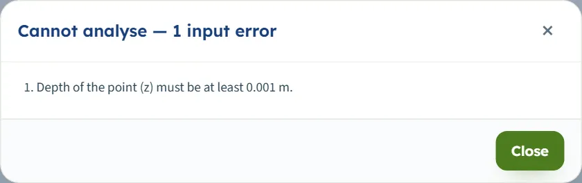
- If you press Analyze, a window titled Cannot analyse — 1 input error (or 2 input errors …) lists each message.
- The limits are shown in the units of the unit system chosen.
| When | Message and what to do |
|---|---|
| The depth is below 0.001 m | “Depth of the point (z) must be at least 0.001 m.” Enter a depth below the surface. |
| The depth is empty | “Depth of the point (z) is missing.” |
| Poisson’s ratio is above 0.5 or below 0 | “Poisson’s ratio (horizontal stresses only) (μ) must be at most 0.5.” or “… at least 0.” |
| A load is negative | “Point load 1 (P1) must be at least 0 kN.” The number of the load is part of the symbol: P2 belongs to load 2. |
| A load or a coordinate is empty | “Point load 1 (P1) is missing.”, “Point A: x on the ground surface (x) is missing.” or “Position of load 1 along x (xL,1) is missing.” |
| The depth of the profile is below 0.1 m or empty | “Depth of the profile (zmax) must be at least 0.1 m.” or “… is missing.” |
When more than one value is wrong the window lists them together, for example “2 input errors” with the depth and Poisson’s ratio.
Messages on the Point loads section
- If you add a load at a position where another already stands, the module says “A point load already stands at this position. Give the new one another position.” and does not add it.
- A load added with a negative or an empty force is entered in the table; the error appears when you press Analyze, for example “Point load 2 (P2) must be at least 0 kN.”
- A load pulled on a drawing onto another load stops at the last free place: “Another point load already stands at this position — the value is kept as it was.”
- Typing a coordinate in the edit form of a load so that it coincides with another load gives the same message and the value reverts.
With usual values the Warnings window reads “No warnings — the assumptions of the solution hold for these inputs.” A negative horizontal stress, which appears under the load axis for μ below 0.5, is a decrease and not a message.
Good practice and common mistakes
- Add the stresses already in the ground. The module gives the increase due to the loads; the effective stress from the weight of the soil is yours to add.
- Use the same coordinates for the loads and for A. The positions xL, yL and the point x, y are on the same ground axes; z is downward.
- Keep the point below the surface. z is at least 0.001 m; at the surface the stress is zero away from the load.
- Pick the vertical stress for settlements and the horizontal ones for the lateral effects you need; Δσz does not depend on μ.
- Let each load be a point. For a footing or an area, a module of that shape gives the stress directly; a point load stands for a load small compared with its distance from A.
- Drag A to explore, type to fix. Dragging is in steps of 5 cm; type the exact coordinates when the design gives them.
- Check the units after switching the system: type values in the units shown beside the boxes.
- Keep a record. The report is the record of an analysis; use Quick Save… or Save to file… to keep the model.
Frequently asked questions
How is the stress below a point load calculated?
By Boussinesq’s solution for an elastic half-space: Δσz = 3P z³ / (2π L⁵) = (P / z²) I1 with L = √(r² + z²) and I1 = (3/2π) / [(r/z)² + 1]5/2. For the module’s example, Δσz = 0.01774 kPa at 6 m below a 5 kN load and 5 m to the side.
Does the result depend on the soil stiffness?
No. The solution does not contain the modulus of elasticity. Poisson’s ratio μ enters the horizontal stresses only; Δσz is the same for any μ.
Is the answer the total stress in the ground?
No, it is the increase caused by the loads. Add it to the stresses already in the ground.
How do I add more loads?
In Point loads fill the New point load form with the force and the position and press Add point load. Up to eight loads; no two at the same place. The stresses of the loads add, and the Calculations tab shows each load and then the sum.
What do the lines of equal stress show?
Lines of equal vertical stress increase in the section: for one load the plane through the load and A, for several loads the plane y = y of A. The blue line is the value at A. The Contours view shows the same field in colour bands on a logarithmic scale.
Can I drag the load and the point on the drawing?
The point A and the dashed profile-depth line can be dragged on the Section and the Contours, before and after Analyze. A load can be dragged before Analyze only: in the 3D view, and, with several loads, along x on the Section and the Contours. After Analyze the loads and Poisson’s ratio are locked until you press Edit inputs.
What happens at the load axis?
The solution is symmetric: r = 0, I1 = 3/(2π) = 0.4775 and Δσz = 0.4775 P/z². The two horizontal stresses are equal there and are zero for μ = 0.5.
What values does the module accept?
The depth of the point at least 0.001 m, Poisson’s ratio from 0 to 0.5, the loads zero or more, the depth of the profile at least 0.1 m, and every box filled. Anything else stops the analysis with a message that names the value.
Which units does it use, and what are the units of the answer?
SI · kN, SI · tf or US, switchable in the header at any time, even after Analyze. The stress is in kPa, t/m² or ksf, the load in kN, tf or kip, and lengths in m or ft. The default example gives 0.01774 kPa, 0.001809 t/m² or 0.0003706 ksf.
What does the report contain?
A cover with your project details and the answer, then six parts: introduction and scope, input data with the section, profile and 3D drawings, the calculation step by step, results, summary and references. It is saved as a PDF or a Word file.
Does the module remember my inputs?
Yes. Every change is kept in the browser, and the page opens again on the model you last worked on, including its analysed state. Reset to defaults brings back the example; Save to file and Quick Save keep copies.
What if the loads are not points?
Use the module of the shape of the load: a line, a strip, a rectangle, a circle, an embankment, or any shape on the Influence chart. For layered ground use the Westergaard modules.