

What the module calculates
Circle, any point gives the increase in vertical stress at any point of the ground below or beside one or several flexible circular areas, each carrying a uniform pressure q on the ground surface: a tank, a silo or a round footing. The ground is taken as a homogeneous, isotropic, elastic half-space. You choose the point A by its position x, y on the ground surface and its depth z, and the module gives Δσz there, the lines of equal stress, the colour contours, the profile with depth under A and a 3D view.
For one circle of radius R the stress at depth z and horizontal distance r from its centre is the integral of Boussinesq’s point-load solution over the loaded area. Ahlvin and Ulery (1962) tabulated it in two parts, A′ and B′, which depend on z/R and r/R only; the module evaluates the integral itself instead of reading a table:
Seen from the point below A, the ray in the direction φ crosses the load between ρ1 and ρ2 (ρ1 = 0 when A is under the load); along each ray the integral is closed, and the sum over φ is done numerically. Directly under the centre (r = 0) it reduces to a closed form:
The module is not limited to the axis: under the circle off its centre, under its edge and beside it it gives the stress at the point you choose, and the result is also given as the influence value A′ + B′ = Δσz/q. With several circles the stress of each is found with its own distance from A, and the stresses are added.
What you can describe
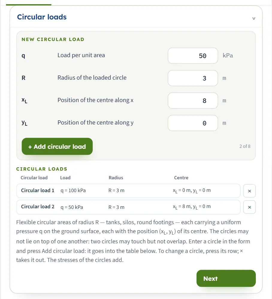
- One to eight circular loads, each with its own load per unit area q, radius R and the position (xL, yL) of its centre on the ground.
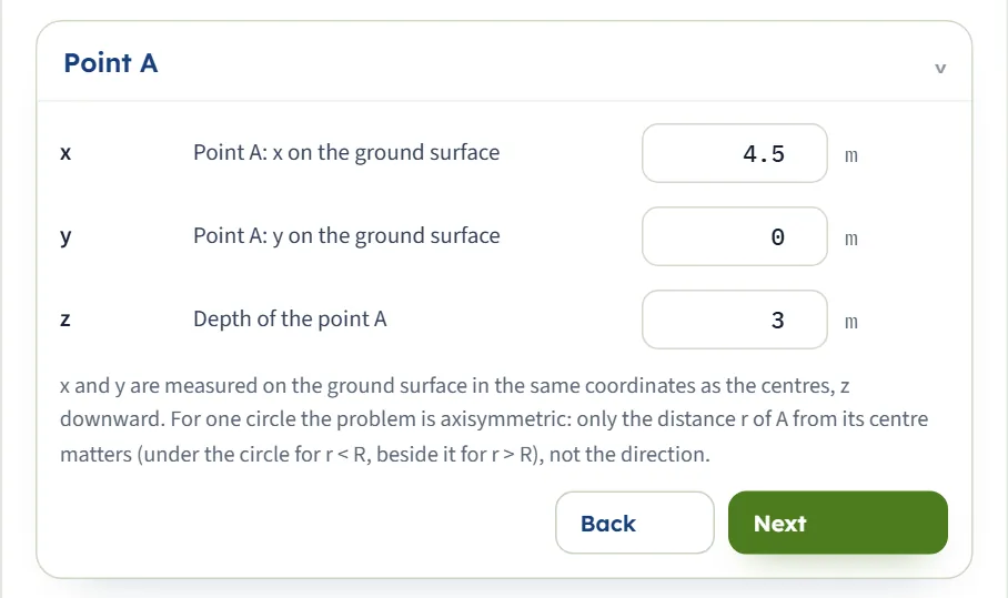
- The point A: its position x, y on the ground surface (the same coordinates as the centres) and its depth z.
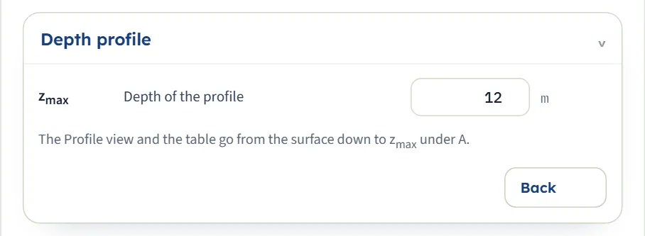
- The depth of the profile zmax, down to which the Profile view and the table under A run.
The result is the increase caused by the circles only; the overburden pressure of the soil above A is not included, so add it to the answer where your design needs the total stress. The module draws the section with the lines of equal stress, colour contours, the profile and a 3D view, writes out the working and prepares a PDF or Word report.
Which module for which load
- A load of rectangular shape in plan: Rectangle. A load of any shape in plan, read from a chart: Influence chart.
- A long strip or an embankment: Vertical strip load, Triangular strip load or Embankment; a concentrated load: Point load.
- A layered ground in which stiff layers spread the load: Westergaard areas.
Before you start: what you need
Have these ready from your design:
| What | Notes |
|---|---|
| The load per unit area q Your design loading | The pressure the circle puts on the ground, zero or more. It is a pressure, not the total force of the tank or silo. |
| The radius R The tank, silo or footing | The radius of the loaded circle, at least 0.001 m; the diameter is 2R. |
| The centre (xL, yL) The layout | The place of the centre on the ground. With one circle you can leave it at 0, 0 and measure A from the centre. |
| The point A: x, y and z Where you want the stress | x and y in the same coordinates as the centres; z at least 0.001 m below the surface. |
Quick start in seven steps
- Open the module and choose the units
Open Circle, any point from the Stresses in a Soil Mass family. Pick SI · kN, SI · tf or US in the header; you can change it at any time.
- Enter the circle
In Circular loads the first circle is already in the table. Press its row to change q, R, xL and yL; or drag the rings at its edges on the Section drawing. To add another circle, fill the New circular load form and press + Add circular load.
- Place the point A
In Point A type x, y and z, or drag the blue point on the Section drawing.
- Set the depth of the profile
In Depth profile type zmax, or drag the dashed line at the foot of the Section drawing.
- Press Analyze
Press Analyze at the foot of the Model tab. The bar reads Analysed and the circles lock; the point A and the profile depth stay free.
- Read the answer
The Results tab gives Δσz at A, the influence value A′ + B′ for one circle, the part from each circle for several, and a table of the stress against depth under A. The lines of equal stress are on the Section drawing, the colour bands in Contours.
- Move A and take the report
Drag A or change x, y and z: the stress there is calculated at once. The Calculations tab writes out the working; the Report tab saves a PDF or a Word file.
The screen: section, contours, profile and 3D
The layout is the one every GeoTerva module shares, described in the workspace guide. For this module the drawing has four views, chosen with the buttons above it:
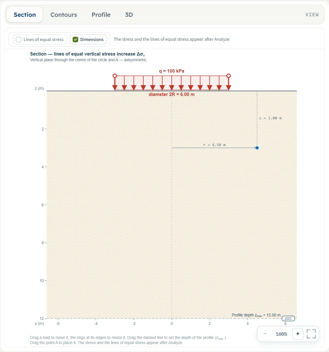
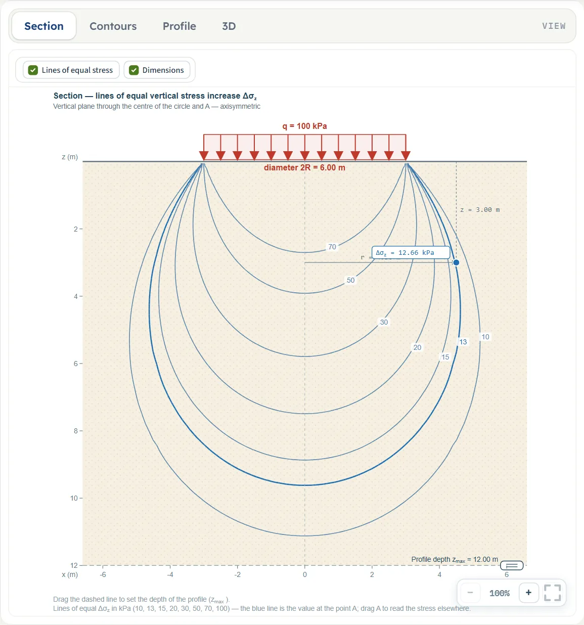
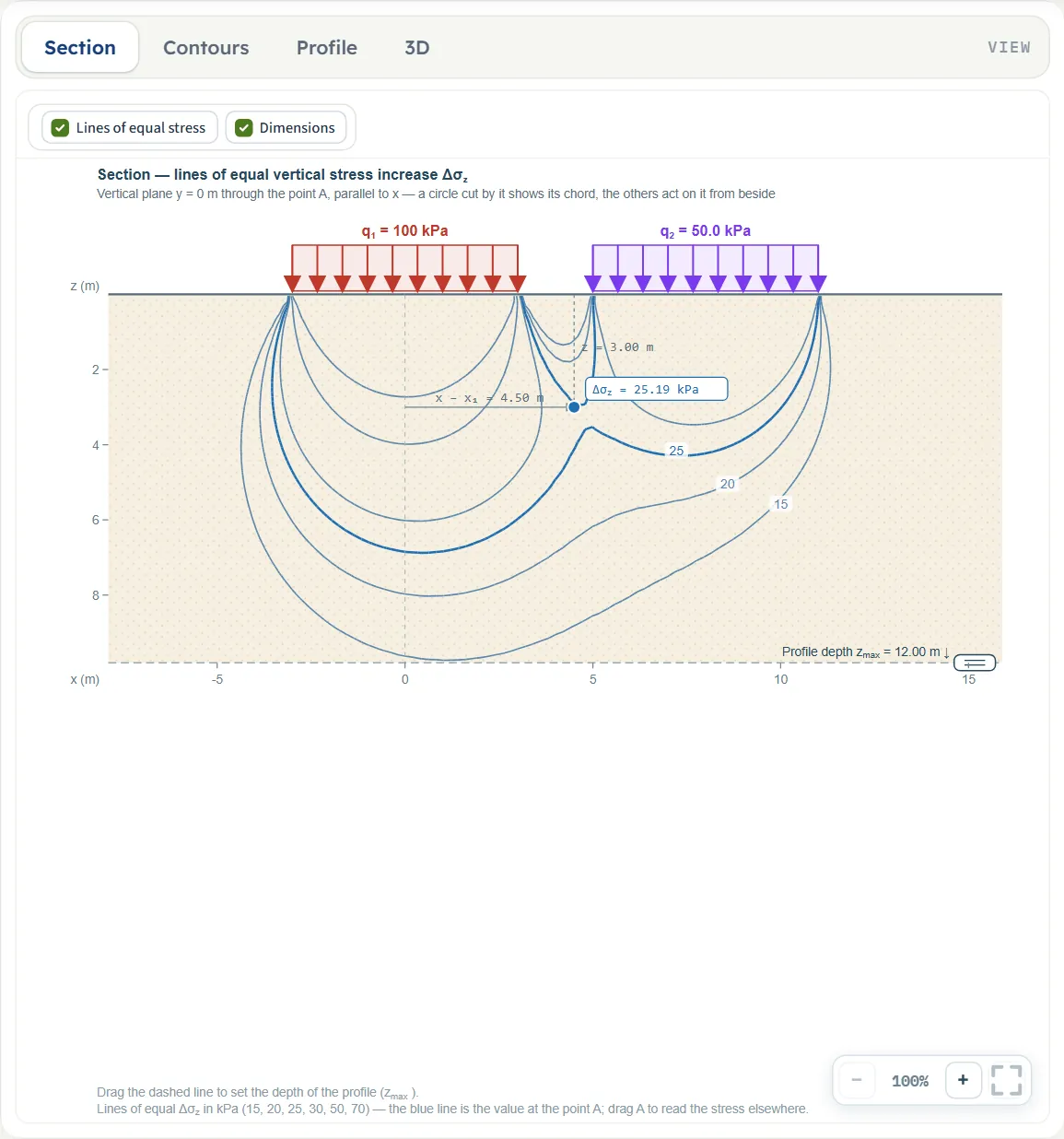
- Section is a vertical section with the loaded circle, the point A, the dimensions r (or x − x1 with several circles) and z and the dashed line of the profile depth. With one circle it is the plane through the centre of the circle and A, and because the problem is axisymmetric the circle is drawn centred on the section. With several circles it is the vertical plane y = yA through A, parallel to the x axis: a circle that this plane cuts shows its chord, and the others act on it from beside. After Analyze it adds the lines of equal stress and a label with Δσz at A.
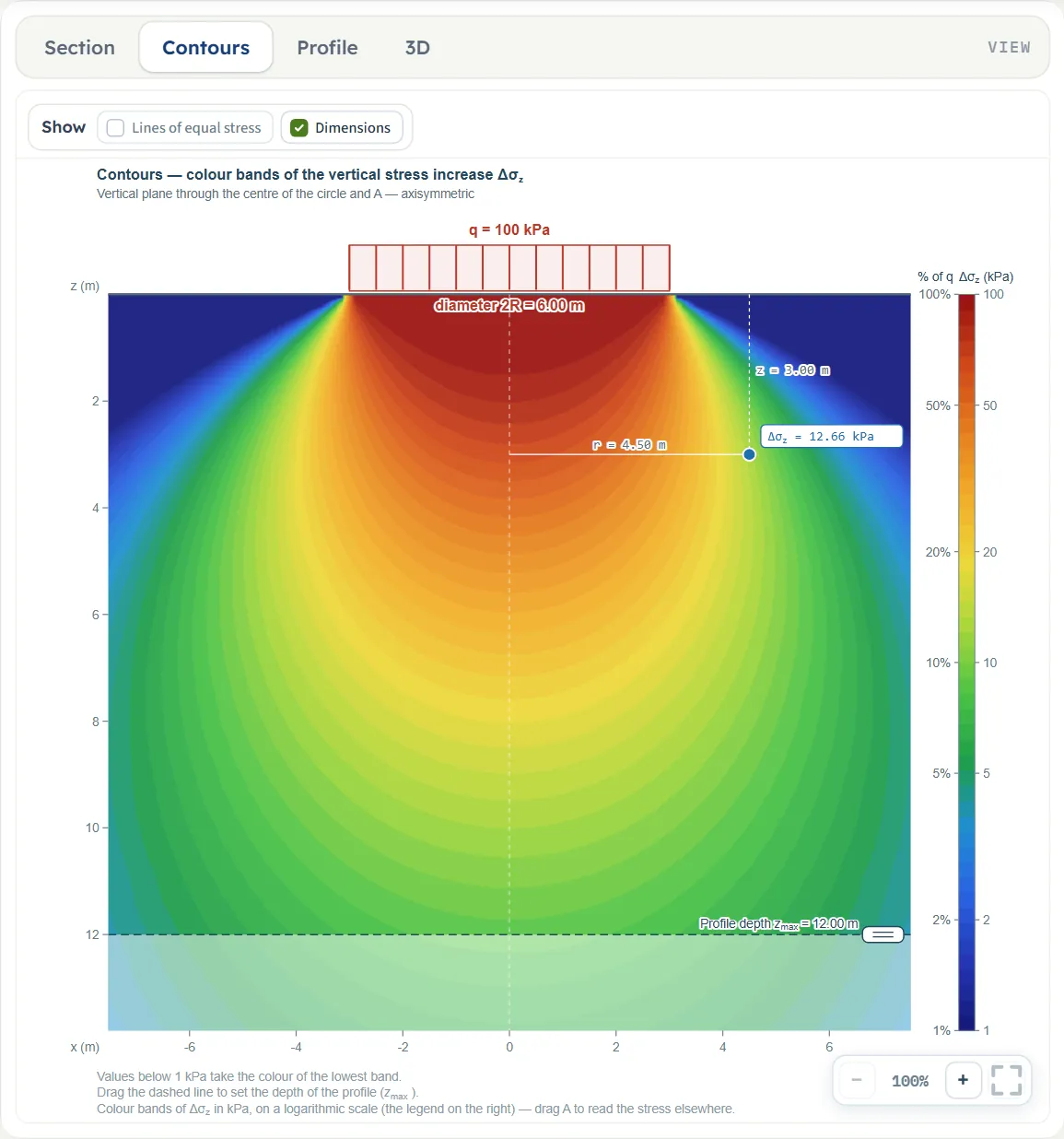
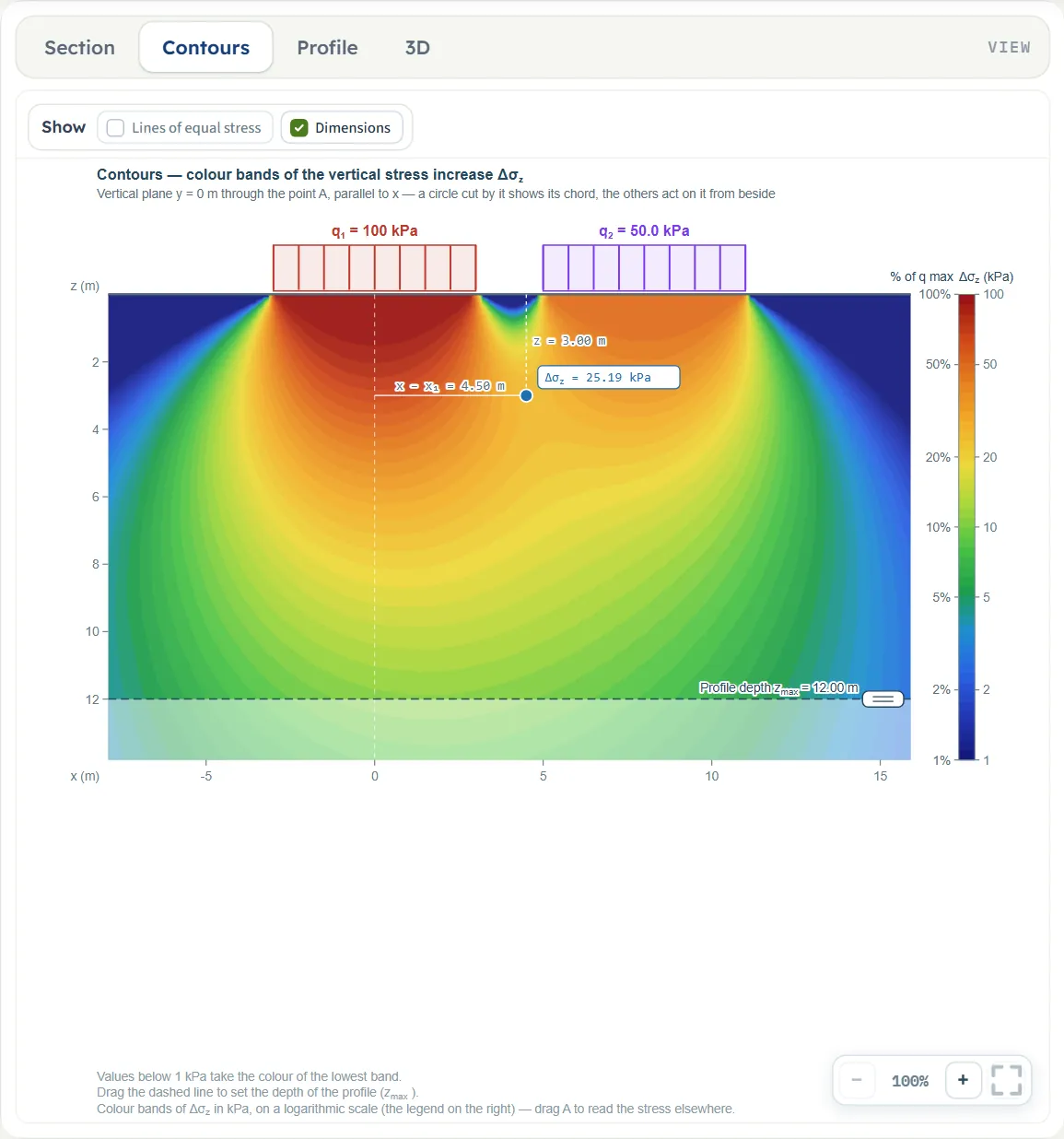
- Contours is the same section filled with colour bands of Δσz on a logarithmic scale, with a legend in kPa and in per cent of q; values below 1 kPa take the colour of the lowest band, and the part below zmax is paler.
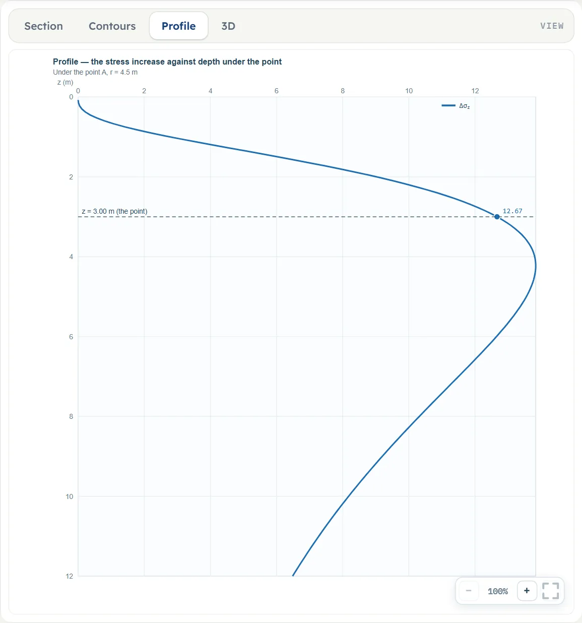
- Profile is the curve of Δσz against depth under A, with a marker at the depth of A.
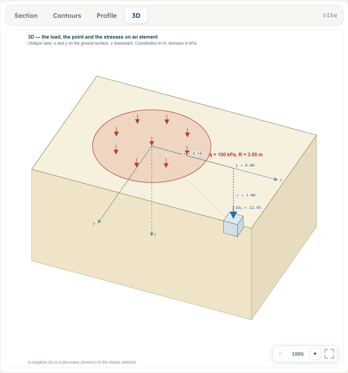
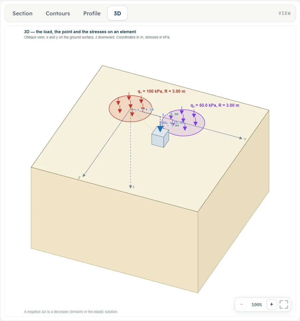
- 3D is an oblique view of the circular load on the ground, the axes x, y and z, and a small element at A with the stress on it.
Before Analyze the drawings follow the inputs and say “The stress and the lines of equal stress appear after Analyze” (Section), “The colour contours of the stress appear after Analyze” (Contours), “The profile appears after Analyze.” (Profile) or “The stresses on the element appear after Analyze.” (3D).
The Show chips
Above the Section and the Contours drawings a bar has two chips: Lines of equal stress and Dimensions. In the Section view the lines chip is off and greyed out until you press Analyze, and then turns on; in Contours it is off by default, so that the lines can be laid over the colours. Dimensions is on by default in both. The Profile and 3D views have no chips. The levels of the lines are listed under the drawing (10, 13, 15, 20, 30, 50, 70 and 100 kPa for the example); the blue line takes the rounded value at A, here 13, and the levels change with the model.
Dragging on the drawing
The hint under the Section drawing reads: “Drag a load to move it, the rings at its edges to resize it. Drag the dashed line to set the depth of the profile (zmax).” What each pull does, as the module runs it, before Analyze (steps of 5 cm):
- One circle, Section view. Drag a ring at the left or right edge of the circle to change the radius: both rings move together, and the centre stays where it is. Pulling the right ring 1 m outward changes R from 3 to 4. The radius stops at 0.1 m. The circle cannot be moved in this view; use the boxes or the 3D view.
- Several circles, Section view. A bar over each circle, as wide as its chord, moves that circle along x: xL follows the pointer. The rings are not shown; change R in the table or in the 3D view.
- 3D view. Drag the disc of a circle over the ground to move it: xL and yL follow the pointer (a short pull, for example 30 px right and 12 px down, moved the example circle to xL = 0.8, yL = 0.15). Drag one of the four rings on its edge to change R; the centre stays.
- Circles never overlap. A pull that would put a circle on another stops at the last free place, where the circles touch, and a message says “That would put circular load 1 and circular load 2 on top of one another — the value is kept as it was.” Circles that touch are allowed.
- The point A. Drag the blue point: z follows the pointer, and so does the position. With one circle the pull changes the distance r from the centre and keeps the direction of A from it: with the centre at (xL, yL) = (3, 4) and A at (x, y) = (6.6, 6.7), a pull of 1 m to the right and 1 m down gave (x, y) = (7.4, 7.3) and z = 4, which is r = 5.5 on the same ray. Pulled to the other side of the axis it gives the same distance as a positive number. With several circles the pull changes x and z and keeps y. The depth stops at 0.05 m at the top and the position at the sides of the drawn frame.
- The dashed line. Drag it up or down to set zmax; it stops at 0.5 m.
- After Analyze the circles are locked, and their rings, bars and discs are gone. The point A and the dashed line stay free, and so do the boxes x, y, z and zmax.
The 3D view has its own hint, “Drag a load over the ground to move it, the rings at its edges to resize it.”
Zoom
Each view has −, a percentage and + at the lower right, and a button that fits the whole drawing in the pane. Zoom changes the drawing on the screen only.
Entering the model, section by section
The Model tab has four sections: Model data, Circular loads, Point A and Depth profile. Each opens when you click its title; Next and Back at the foot walk you through them, and Analyze waits below the last one. Where a unit is shown twice or three times, such as m · ft, the units are those of SI · kN, SI · tf and US in turn, and equal ones are merged. Defaults are shown in SI; in other unit systems the boxes show the converted values with their unrounded digits, for example 9.84252 ft for the 3 m radius and 10.1972 t/m² for 100 kPa.
Model data
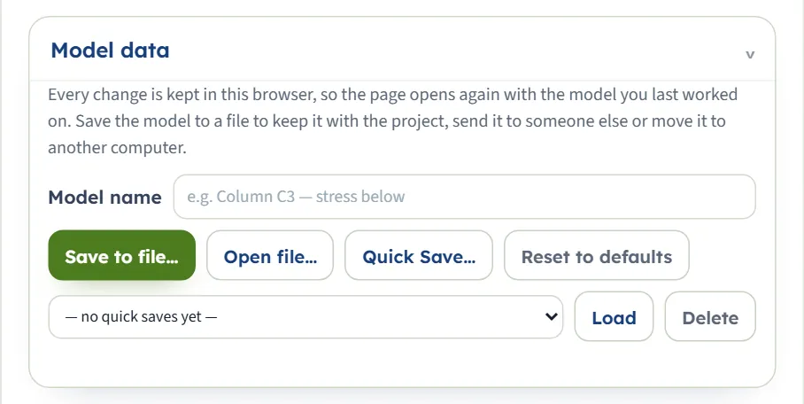
The first section holds the model name, Save to file…, Open file…, Quick Save… with its list and Load and Delete, and Reset to defaults. It works as described in the workspace guide.
Circular loads
The section is a form over a table. The New circular load form takes q, R, xL and yL; + Add circular load puts the circle into the Circular loads table, and a counter beside the button shows how many of the eight circles there are. The table lists each circle with its load, radius and centre. Press a row to change that circle in the form (the form then reads Editing · Circular load 1 and offers Done and Delete circular load; the note says that changes apply as they are entered), or press × to take a circle out. The first circle is already in the table when the module opens, and × is greyed out while it is the only one.
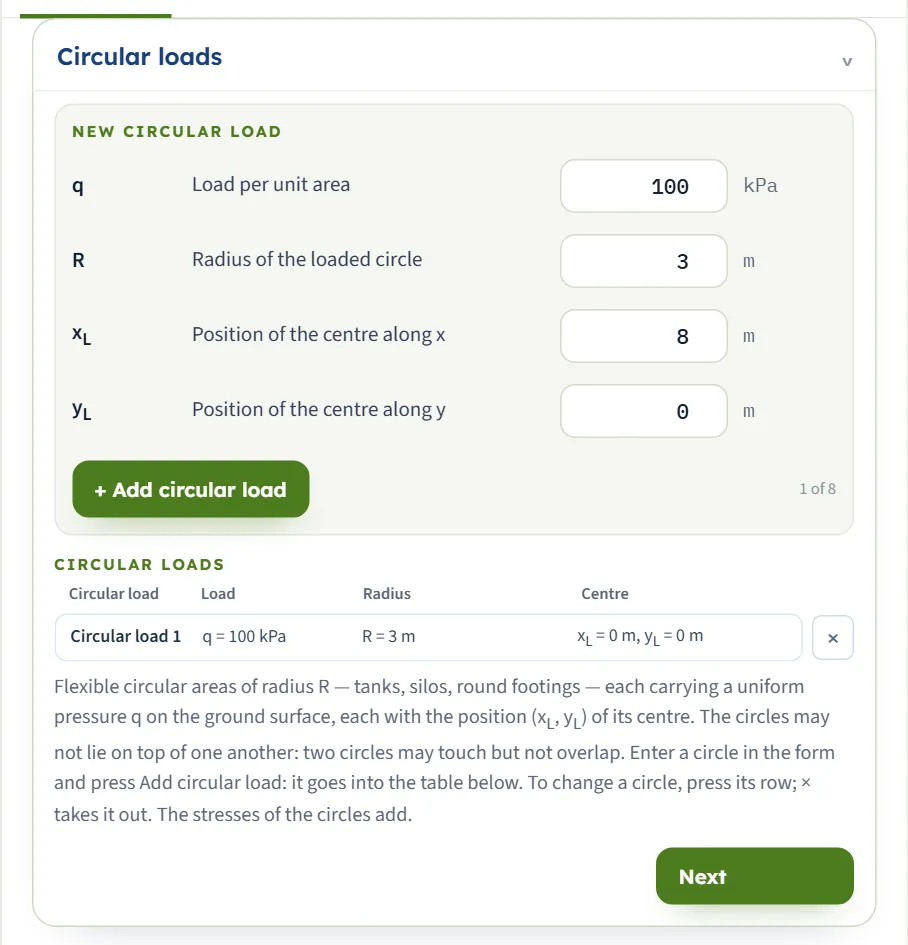
| Field | Default | What to enter |
|---|---|---|
| Load per unit area q kPa · t/m² · ksf | 100 | The uniform pressure of the circle on the ground. Zero or more. |
| Radius of the loaded circle R m · ft | 3 | At least 0.001 m. |
| Position of the centre along x xL m · ft | 0 (circle 1) · 8 (form) | On the ground, in the coordinates of the point A. Circle k of a model made by the module starts at 8 × (k − 1); the New circular load form opens with 8. |
| Position of the centre along y yL m · ft | 0 | On the ground, in the coordinates of the point A. |
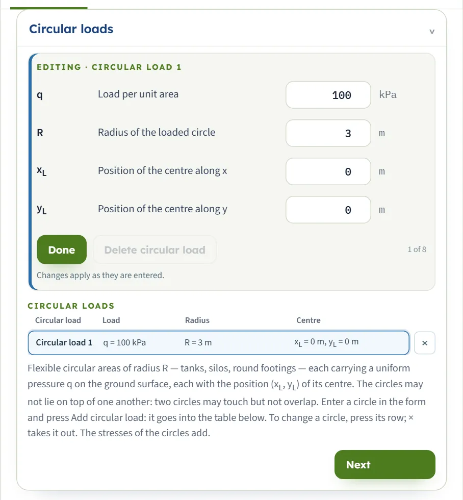
The circles may not lie on top of one another: two circles may touch but not overlap, that is, the distance between their centres is at least the sum of their radii. Adding or editing a circle that would overlap another is refused (see Messages). The circles are numbered in the order you add them, and the numbers name the results “From circular load 1”, “From circular load 2” and so on.
Point A
The three coordinates of the point where you want the stress. A is under the ground surface at the position x, y and the depth z. The note in the section says that x and y are measured on the ground surface in the same coordinates as the centres and z downward, and that for one circle the problem is axisymmetric: only the distance r of A from its centre matters, under the circle for r < R and beside it for r > R, not the direction.
| Field | Default | What to enter |
|---|---|---|
| Point A: x on the ground surface x m · ft | 4.5 | In the coordinates of the centres. For one circle only the distance from its centre counts. |
| Point A: y on the ground surface y m · ft | 0 | In the coordinates of the centres. |
| Depth of the point A z m · ft | 3 | At least 0.001 m below the ground surface. |
Depth profile
The depth down to which the Profile view and the table of the stress under A run.
| Field | Default | What to enter |
|---|---|---|
| Depth of the profile zmax m · ft | 12 | At least 0.1 m. The Profile view and the table under A go from the surface down to this depth, or to the depth of A if that is deeper. |
One circle, several circles and where A is
The one choice in the module is how many circles there are, from 1 to 8; you make it by adding or deleting circles. The stress of each circle is found as if it were alone, with the distance r of A from its centre, and the stresses are added. This works because the ground is elastic, so the stresses of separate loads add.
- Only the distance counts for one circle. The stress depends on r, z and R. Moving the centre to (xL, yL) = (3, 4) and A to (6.6, 6.7) keeps r = 4.5 m and gives 12.66 kPa, the same as the example (12.66 kPa); so does A at (x, y) = (0, 4.5) with the circle at the origin (12.66 kPa), and A at x = −4.5 on the other side (12.66 kPa).
- Under, at the edge, beside. With z = 3 m and R = 3 m the module gives 64.64 kPa at r = 0, 60.92 kPa at 1 m, 33.22 kPa under the edge (r = R), 12.66 kPa at 4.5 m, 4.181 kPa at 6 m and 0.04884 kPa at 15 m.
- Loads and radii can differ. Each circle has its own q and R, so a tank and a smaller silo beside it can be put in one model.
- The cards show the parts. The Results tab shows the total and the part from each circle, and the Calculations tab writes out each circle’s working.
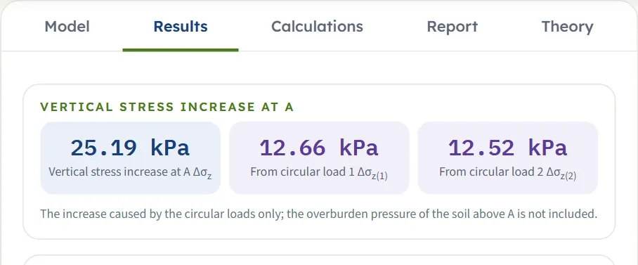
With the example circle (100 kPa, radius 3 m, at the origin) and A at (x, y, z) = (4.5, 0, 3), a second circle of 100 kPa and radius 3 m centred at xL = 8 m gives the total 37.71 kPa: 12.66 kPa from the first and 25.05 kPa from the second, whose centre is 3.5 m from A. If the second circle carries 50 kPa, its part is 12.52 kPa and the total is 25.19 kPa. A point midway between two such circles (xL = 0 and 8 m, A at x = 4 m) gets 36.15 kPa, and with the circles touching (xL = 0 and 6 m, A at x = 3 m, the point of contact) 66.45 kPa.
Which should I use?
- One circle or several? One circle for a tank, silo or round footing on its own; several circles for a group of tanks, or for round loads of different pressures side by side.
- A load that is not round is not several circles: use Rectangle for a rectangular footing, or Influence chart for any shape in plan.
- A load that is long compared with its width is closer to a strip: use Vertical strip load.
Analyze and read the results
Press Analyze. The bar changes to Analysed — the stress at the point calculated and says “The inputs are locked. Edit inputs clears the results; the unit system can still be changed. The point A stays free: drag it on the drawing or change its coordinates, and the stress there is calculated at once.” A message appears briefly, “Analysed — see the Results tab and the Calculations.” The module stays on the Model tab: open Results for the answer. The Section view now shows the lines of equal stress.
| Card | Symbol | The example |
|---|---|---|
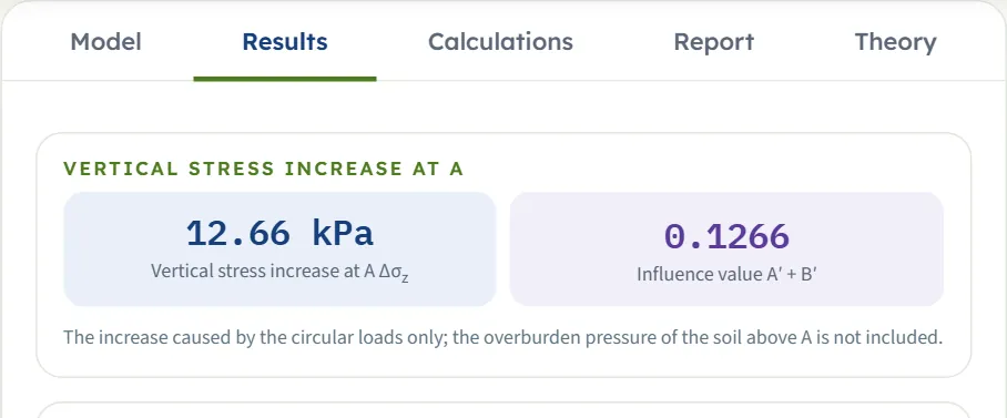
| Vertical stress increase at A | Δσz | 12.66 kPa |
| Influence value (one circle) | A′ + B′ | 0.1266 |
| From circular load k (several circles) | Δσz(k) | part of the total from circle k |
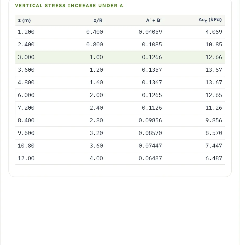
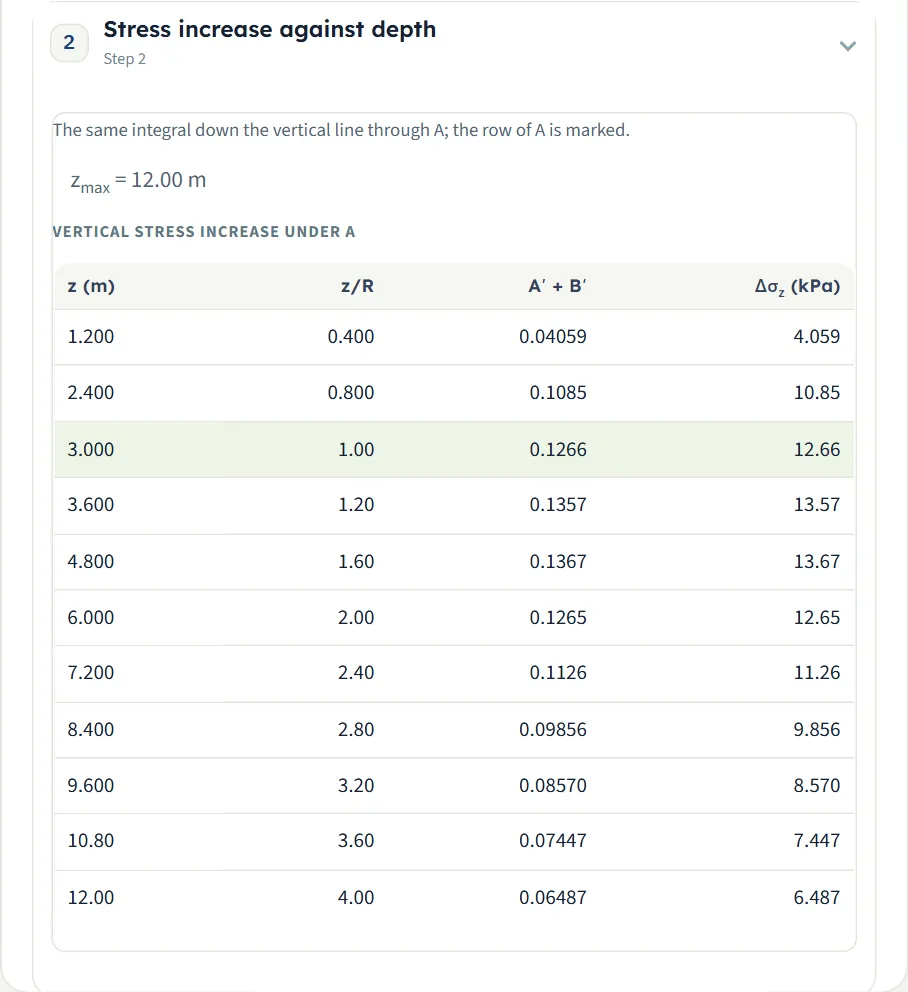
Below the cards the Vertical stress increase under A table gives z, Δσz and, for one circle, z/R and A′ + B′ at ten equal steps down to zmax, with the row of A inserted and highlighted. The Profile view runs a little deeper than A if zmax is smaller than the depth of A. With several circles the table has z and Δσz only, and the card of the influence value is replaced by the part from each circle. A Values, step by step table above it lists the steps of the Calculations tab with their values.
Using the numbers
- The result is an increase, not the total stress: add the overburden pressure of the soil above A for the total vertical stress.
- The influence value A′ + B′ is the part of the surface pressure that reaches A. It is 1 on the surface under the circle and falls with depth on the axis; beside the circle it first rises with depth and then falls (for the example, 4.059 kPa at 1.2 m, 12.66 kPa at 3 m, 13.67 kPa at 4.8 m and 6.487 kPa at 12 m).
- The curve in the Profile view is summed over fewer directions than the card, so its last digit can differ by one: the marker at A reads 12.67 where the card says 12.66 (an independent integration gives 12.665).
- Change x, y or z after Analyze and everything follows at once; to change a circle, press Edit inputs, which unlocks the circles and clears the results.
- Changing the unit system after Analyze re-states the cards and the report without a new run. The drawings keep their labels in m and kPa.
Warnings and notes
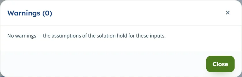
The bar carries a Warnings (0) button. It opens a window that says “No warnings — the assumptions of the solution hold for these inputs.” The runs of this manual, from the example to eight circles, gave no warning.
The Calculations tab, the report and the Theory tab
The Calculations tab opens with Given and what is sought and then writes out the working in numbered steps, ending with the answer. For one circle:
- Stress at A — Δσz = q (A′ + B′), z/R and r/R with your numbers and a note on where A is (“A is outside the loaded circle”, “A is under the loaded circle” or “A is under the edge”), the integral about the point, A′ + B′ and Δσz = A′ + B′ × q, and for comparison the stress on the axis at the same depth. When A is on the axis (r = 0) the closed form is shown first, and the general integral gives the same.
- Stress increase against depth — the same integral down the vertical line through A, as the table of the Results tab, with the row of A marked.
With several circles there is one step for each circle, with its own distance r = √[(x − xL)² + (y − yL)²], then a Superposition step that adds the parts, then the depth table.
The report
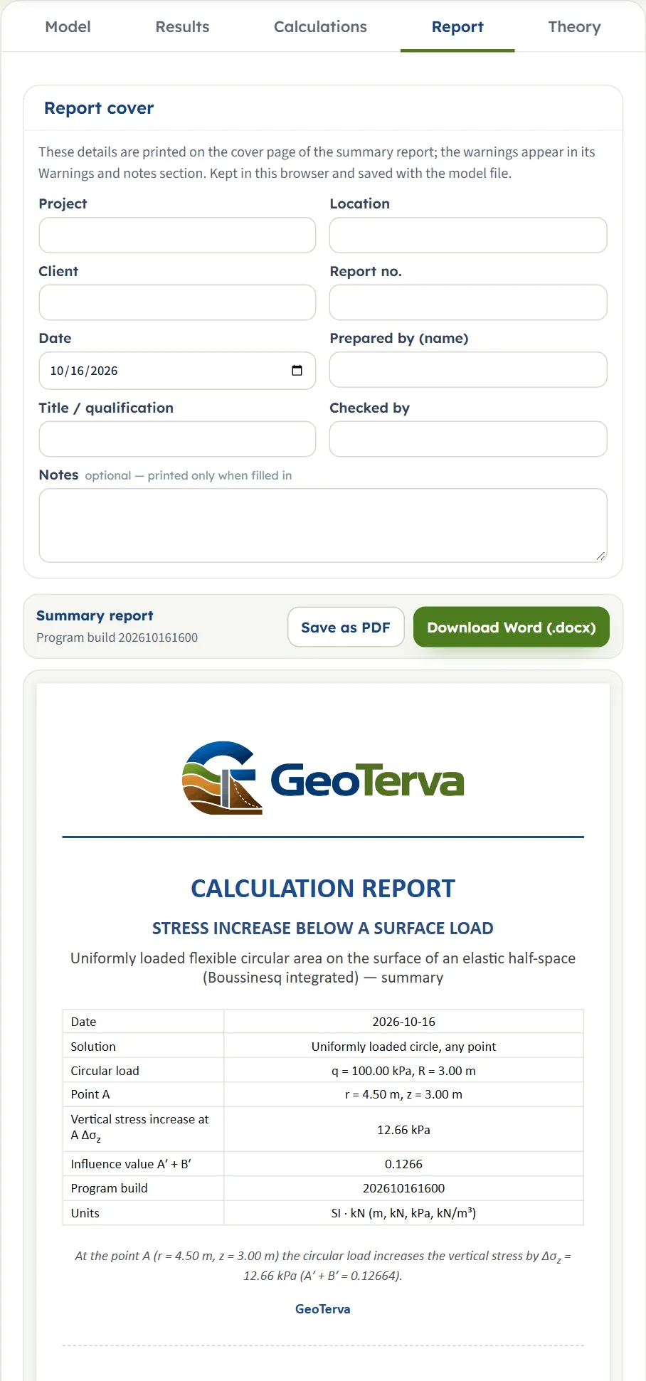
In the Report tab fill in the cover (project, location, client, report number, date, prepared by, title or qualification, checked by, and optional notes). The details are kept in this browser and saved with the model file. Save as PDF and Download Word (.docx) produce the summary report; the preview below the buttons is the report itself.
The report has six parts: 1 Introduction and scope, 2 Input data, 3 Calculation, 4 Results, 5 Summary and 6 References. It carries three drawings, the Section with the lines of equal stress, the Profile and the 3D view, and states the units used.
The Theory tab
The Theory tab has five sections: Scope and assumptions, The solution, How the program computes it, Worked example and References. Each opens when you click its title (Open all and Close all open or close them together). It sets out the closed form on the axis, why there is none elsewhere, the integral that the module evaluates and a table of A′ + B′ at several values of z/R and r/R; the figures in it are computed from the equations.
Worked example: the module’s own example
The module opens on this example, so you can follow the numbers on your own screen.
| Section | Input | Value |
|---|---|---|
| Circular loads | Circular load 1 | q = 100 kPa; R = 3 m; centre at 0, 0 |
| Point A | Position and depth | x = 4.5 m; y = 0; z = 3 m |
| Depth profile | Depth | zmax = 12 m |
Step 1: where A is
The distance from the centre is r = 4.5 m, so r/R = 1.5 (A is outside the loaded circle) and z/R = 1.
Step 2: the stress
The integral about the point has no closed form here. Evaluated by the module, A′ + B′ = 0.12664, so Δσz = 0.12664 × 100 = 12.66 kPa. An independent numerical integration of Boussinesq’s point-load solution over the circle, done outside the module, gives 0.12665. For comparison, directly under the centre at the same depth the closed form gives Δσz = 100 × {1 − 1/[(3/3)² + 1]3/2} = 100 × (1 − 0.35355) = 64.64 kPa, about five times the stress at A; the module prints this comparison in step 1 of the Calculations tab.
These are the two cards of the Results tab and the step of the Calculations tab. The same integral at the depths of the table gives the profile: the module’s table gives 4.059 kPa at 1.2 m, 12.66 kPa at 3 m, 13.67 kPa at 4.8 m and 6.487 kPa at 12 m, and the same independent integration gives 4.059, 12.67, 13.67 and 6.487 kPa.
Directly under the centre
Set x = 0 and the point is on the axis. At z = 1.5 m, R/z = 2 and the closed form gives 100 × (1 − 1/53/2) = 100 × (1 − 0.08944) = 91.06 kPa; the module gives 91.06 kPa. At z = 3 m the module gives 64.64 kPa, the 64.64 kPa above, and at z = 12 m 8.692 kPa, where R/z = 0.25 and 100 × (1 − 1/1.06253/2) = 8.69 kPa by hand.
Other unit systems
The same circle in SI · tf, with q = 10 t/m² (the other values unchanged), gives 1.266 t/m² and the influence value 0.1266. In US the default example, which is 2.089 ksf on a circle of 9.843 ft radius, gives 0.2645 ksf: the same circle and point as 12.66 kPa. A check by hand with round US numbers: q = 2 ksf, R = 10 ft, A at x = 15 ft, z = 10 ft has the same z/R = 1 and r/R = 1.5, so the influence value is 0.12664 and Δσz = 0.12664 × 2 = 0.2533 ksf; the module gives 0.2533 ksf. In SI · tf, q = 10 t/m², R = 2 m, x = 3 m, z = 2 m again has the ratios 1 and 1.5 and gives 1.266 t/m²; the module gives 1.266 t/m².
How each input changes the answer
Each row changes one thing in the example (one circle of q = 100 kPa, R = 3 m at the origin, A at x = 4.5 m, y = 0, z = 3 m) and runs the module again, in SI · kN. The numbers are the ones the module gives, so you can reproduce any row; an independent numerical integration of the point-load solution agrees with every row.
| Change | Δσz (kPa) |
|---|---|
| The example A′ + B′ = 0.1266 | 12.66 |
| q = 200 kPa The stress is proportional to the load; the influence value is unchanged A′ + B′ = 0.1266 | 25.33 |
| q = 50 kPa Half the load, half the stress A′ + B′ = 0.1266 | 6.332 |
| R = 1.5 m A smaller circle: A is now 3 m outside its edge, and the stress falls A′ + B′ = 0.02250 | 2.250 |
| R = 2 m A smaller circle puts less on the same point A′ + B′ = 0.04411 | 4.411 |
| R = 4 m A larger circle: A is now 0.5 m outside its edge A′ + B′ = 0.2842 | 28.42 |
| R = 6 m A is now under the circle, 1.5 m inside its edge A′ + B′ = 0.6923 | 69.23 |
| R = 20 m A is deep inside a very large circle: the stress approaches q A′ + B′ = 0.9961 | 99.61 |
| x = 0 (on the axis) The closed form applies; the highest stress at this depth A′ + B′ = 0.6464 | 64.64 |
| x = 1 m Under the circle, 2 m inside its edge A′ + B′ = 0.6092 | 60.92 |
| x = 2 m Under the circle, 1 m inside its edge A′ + B′ = 0.4971 | 49.71 |
| x = 3 m (under the edge) At the edge: about one third of q at this depth A′ + B′ = 0.3322 | 33.22 |
| x = 4 m 1 m outside the edge A′ + B′ = 0.1808 | 18.08 |
| x = 6 m Beside the circle, 3 m from the edge A′ + B′ = 0.04181 | 4.181 |
| x = 9 m Farther out A′ + B′ = 0.006246 | 0.6246 |
| x = 15 m Far from the circle the stress is a tiny part of the load A′ + B′ = 0.0004884 | 0.04884 |
| z = 0.01 m At the surface beside the circle the stress is nearly zero A′ + B′ = 0.00000005 | 0.00000451 |
| z = 0.5 m Close to the surface, beside the circle A′ + B′ = 0.004918 | 0.4918 |
| z = 1.5 m Beside the circle the stress rises with depth at first A′ + B′ = 0.06044 | 6.044 |
| z = 6 m Past the largest value, which is at about 4.2 m for this point: the stress now falls A′ + B′ = 0.1265 | 12.65 |
| z = 9 m The stress keeps falling A′ + B′ = 0.09194 | 9.194 |
| z = 12 m Four radii deep A′ + B′ = 0.06487 | 6.487 |
| x = 3 m, z = 3 m Under the edge at a depth equal to the radius A′ + B′ = 0.3322 | 33.22 |
| xL = 3 m (A at x = 4.5 m) A is 1.5 m from the centre: under the circle A′ + B′ = 0.5622 | 56.22 |
| R = 6 m, z = 6 m, x = 9 m Every length doubled: the same z/R and r/R, the same stress as the example A′ + B′ = 0.1266 | 12.66 |
Several circles, SI · kN, added to the example (A at x = 4.5 m, y = 0, z = 3 m unless the row says otherwise):
| Added | Total (kPa) | Parts (kPa) |
|---|---|---|
| Circle 2: 100 kPa, R = 3 m, centre at xL = 8 m The centre of circle 2 is 3.5 m from A | 37.71 | 12.66 + 25.05 |
| Circle 2: 50 kPa, R = 3 m, centre at xL = 8 m | 25.19 | 12.66 + 12.52 |
| Circle 2: 100 kPa, R = 3 m, centre at xL = 6 m The circles touch at x = 3 m | 68.89 | 12.66 + 56.22 |
| Circle 2: 200 kPa, R = 1.5 m, centre at xL = 6 m A smaller, more heavily loaded circle | 51.86 | 12.66 + 39.20 |
| Circle 2: 100 kPa, R = 3 m, centre at yL = 6 m Beside the first along y; A stays at y = 0 | 14.17 | 12.66 + 1.510 |
| Circles 2 and 3: 100 kPa, R = 3 m, centres at xL = 8 m and 16 m | 37.90 | 12.66 + 25.05 + 0.1850 |
The pattern follows the integral. The stress is proportional to q; it depends on z/R and r/R only, so doubling every length leaves it unchanged; on the axis it falls steadily with depth, while beside the circle it rises to a largest value and then falls; and with z near zero it equals q under the circle and zero beside it. The depth of the profile zmax changes the table and the Profile view but not the stress at A: 12.66 kPa with zmax = 6 m and 12.66 kPa with zmax = 0.5 m, a depth the module extends to the depth of A.
Messages: when the module stops, and what it notes
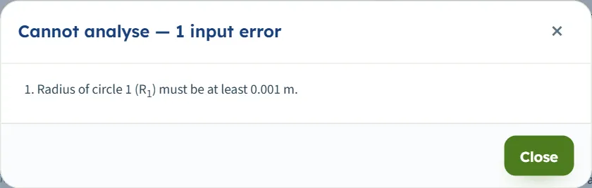
The module checks the numbers it needs before it calculates. When an input cannot be used, press Analyze and a window titled Cannot analyse — 1 input error (or 2 input errors …) lists each message; a box whose value is outside its limit is marked in red. Nothing is calculated.
| When | Message and what to do |
|---|---|
| R is 0 | “Radius of circle 1 (R1) must be at least 0.001 m.” Enter a radius of at least 0.001 m. |
| q is negative | “Load per unit area of circle 1 (q1) must be at least 0 kPa.” Enter zero or a positive load. |
| z is 0 | “Depth of the point A (z) must be at least 0.001 m.” Enter a depth of at least 0.001 m. |
| zmax is 0 | “Depth of the profile (zmax) must be at least 0.1 m.” Enter a depth of at least 0.1 m. |
| A box is empty | “Radius of circle 1 (R1) is missing.” or “Point A: x on the ground surface (x) is missing.” Fill the box or take the circle out. |
| Two values are wrong | The window reads “Cannot analyse — 2 input errors” and lists both: “Radius of circle 1 (R1) must be at least 0.001 m. Depth of the point A (z) must be at least 0.001 m.” |
| A new circle would overlap another | A message appears briefly: “The new circular load would lie on circular load 1 — they cannot overlap. Give it another position or width.” The circle is not added. |
The messages use the numbered names of the circles, such as “circle 1” and “R1”, even when there is only one circle, and the limits in the units of the unit system chosen. When you type a position or radius into a circle already in the table and it would put two circles on one another, a message appears briefly: “That would put circular load 1 and circular load 2 on top of one another — the value is kept as it was.” and the value stays as it was. A radius that is too big does the same. At eight circles + Add circular load is greyed out and the counter reads 8 of 8.
Notes and warnings
With every input inside its limits the module calculates, and the Warnings window reads “No warnings — the assumptions of the solution hold for these inputs.” A load of zero is accepted and gives 0 kPa, with a dash for the influence value. Large values are accepted too: with q = 1,000,000 kPa and R = 1000 m, a circle that is nearly infinite in extent around A, the module gives 1,000,000 kPa, an influence value of 1.000.
Good practice and common mistakes
- Use the module for a loaded circle on the ground. The circle is flexible, so the pressure stays q across it. A stiff footing distributes its pressure differently; the module gives the stress for the pressure you enter.
- Enter a pressure, not a force. q is a load per unit area. For a tank, divide the total weight, content included, by the area of the circle, πR².
- Use the radius, not the diameter. The drawing labels the diameter 2R so that you can check it.
- Mind the coordinates. x, y and the centres are in the same coordinates on the ground; with one circle only the distance between A and the centre matters, with several the position of A counts.
- Do not overlap circles. Circles may touch but not lie on one another; the module does not take a circle inside another.
- Add the overburden. The result is the stress increase; for the total vertical stress add the soil weight above A.
- Read the profile with the radius in mind. Under the centre the stress is 64.64 kPa of 100 at one radius of depth and falls steadily below; beside the circle it first rises: for A at 4.5 m from the centre the largest value, about 13.8 kPa, is at a depth of about 4.2 m.
- Place A with the drawing, then type exact values. Dragging snaps to 5 cm; type the coordinates when you need a given place.
- Check the units after switching the system: type values in the units shown beside the boxes.
- Keep a record. The report is the record of an analysis; use Quick Save… or Save to file… to keep the model.
Frequently asked questions
How is the stress below a circular load calculated?
The module integrates Boussinesq’s point-load solution over the loaded circle, in polar coordinates about the point below A. The result is Δσz = q (A′ + B′), with A′ + B′ depending on z/R and r/R only, where r is the horizontal distance of A from the centre. For the module’s example it gives 12.66 kPa.
Does it work only under the centre of the circle?
No. Directly under the centre there is a closed form, which the module shows first when A is on the axis; at any other point, under the circle off its centre, under its edge or beside it, the module evaluates the integral itself. The example point is 1.5 m beside the edge of the circle.
What is the influence value A′ + B′?
It is the stress increase divided by the pressure of the circle. It depends only on z/R and r/R, and it is the number to use if you have a table of influence values. The module gives it for one circle; with several circles it gives the stress of each.
Does the result include the weight of the soil?
No. It is the increase caused by the circles only. Add the overburden pressure of the soil above A for the total vertical stress.
How many circles can I add, and can they overlap?
Up to eight, each with its own q, R and centre. They may touch but not overlap; the module refuses a circle that would lie on another. The stresses of the circles add.
Can I drag the circle and the point on the drawing?
Yes, before Analyze. In the Section view of one circle, the rings at its edges change the radius; with several circles a bar over each circle moves it along x; in the 3D view you drag the disc to move it and the rings to change the radius. The blue point places A and the dashed line sets the depth of the profile; they move in 5 cm steps. After Analyze the circles are locked, but A and the dashed line stay free.
What does the point A depend on?
On x, y and z. With one circle, only on the distance r of A from the centre and on z: the stress is the same on every point of the same circle around the axis. With several circles the position of A relative to each centre counts.
What do the lines of equal stress show?
Each line joins the points of the section with the same Δσz, labelled in kPa; the line through A is blue. Switch them on and off with the Lines of equal stress chip. The Contours view shows the same stress as colour bands on a logarithmic scale.
What values does the module accept?
q zero or more, R at least 0.001 m, z at least 0.001 m, zmax at least 0.1 m, and x, y and the centres any value. Anything else stops the analysis with a message that names the value.
Which units does it use, and what are the units of the answer?
SI · kN, SI · tf or US, switchable in the header at any time, even after Analyze. Stresses are in kPa, t/m² or ksf and lengths in m or ft. The default example gives 12.66 kPa; in US, 0.2645 ksf. A circle of 10 t/m² gives 1.266 t/m² in SI · tf.
What does the report contain?
A cover with your project details and the answer, then six parts: introduction and scope, input data, the calculation step by step, results, summary and references, with the section, profile and 3D drawings. It is saved as a PDF or a Word file once the model is analysed.
Does the module remember my inputs?
Yes. Every change is kept in the browser, and the page opens again on the model you last worked on, including its analysed state. Reset to defaults brings back the example; Save to file and Quick Save keep copies.
When is a circle the wrong model?
When the loaded area is not round: use Rectangle for a rectangular footing or Influence chart for any other shape. When the load is a long band: use Vertical strip load.