

What the module calculates
Horizontal strip load gives the vertical stress increase at a point in the ground below one or several flexible strips of finite width and infinite length that carry a uniform load pushing along the ground surface (a horizontal load) or at an angle to the vertical (an inclined load). The ground is a homogeneous, isotropic, linearly elastic half-space and the problem is plane strain: every cross-section along the strip is the same. Such loads are the friction under a sliding footing, the thrust at the base of a retaining wall or the braking of vehicles on a road.
An inclined load of pressure q at the angle α from the vertical is split into a vertical part qv and a horizontal part qh, each is solved apart, and the two stresses add. With b = B/2 and x the horizontal distance of the point A from the centre line of the strip:
ω is the angle that the strip subtends at A and δ is the angle between the vertical through A and the line from A to the edge of the strip on the +x side (signed; negative when A is under the strip). The horizontal part is odd in x: it raises the stress ahead of the load (+x for a load that pushes toward +x) and lowers it behind, and it is zero under the centre line. For several strips each strip is taken with its own x, the distance of A from its centre line, and the stresses are summed.
What you can describe
- One to eight strips. Each has its own load per unit area q, inclination α from the vertical (from −90° to 90°; 0° is a vertical strip, 90° a purely horizontal one), width B and the position xc of its centre line along the ground. Strips may meet at an edge but may not overlap.
- A point A at the horizontal position x and the depth z.
- The depth of the profile zmax: how deep the Profile view and the table under A go.
The module gives the vertical stress increase at A, its vertical and horizontal parts, and, for two or three strips, the part of each strip. It draws the lines of equal stress, the colour contours, the stress against depth under A and a 3D view, writes out the working, and prepares a PDF or Word report. The increase is the one caused by the strip loads only; the overburden pressure is not included, and a negative value is a decrease.
Which module for what
- A strip loaded vertically only: Vertical strip load. Here, α = 0° gives the same loading and the horizontal part is zero.
- A load of no width: Horizontal line load takes horizontal or inclined line loads.
- A strip whose load rises linearly from zero at one edge: Triangular strip load; a long embankment with side slopes: Embankment.
- Loaded circles and rectangles: Circle, any point and Rectangle.
Before you start: what you need
Have these ready from your design:
| What | Notes |
|---|---|
| The load of each strip | The pressure q per unit area, and its inclination α from the vertical: how much of it is vertical and how much pushes along the surface. |
| The width B of each strip | Measured across the strip, in the plane of the section. The strip is infinitely long in the other direction. |
| The position xc of each centre line | Along the same axis as the point A. The first strip is at 0 unless you move it. |
| The point A: x and z | The horizontal position along the same axis, and the depth below the surface. |
| The depth of the profile zmax | The table runs from the surface to zmax (to the depth of A instead, if A is deeper), and the Profile view shows at least zmax. |
Quick start in seven steps
- Open the module and choose the units
Open Horizontal strip load from the Stresses in a Soil Mass family. Pick SI · kN, SI · tf or US at the top right; you can change it at any time.
- Describe the strips
In Strip loads the first strip is already in the table. Press its row to change its load q, inclination α, width B and centre line xc in the form, or fill the New strip load form and press + Add strip load for more.
- Place the point A
In Point A type the horizontal position x and the depth z. You can also drag A on the drawing.
- Set the depth of the profile
In Depth profile type zmax.
- Press Analyze
Press Analyze in the bar at the foot of the Model tab. The bar reads Analysed — the stress at the point calculated, the strips lock, and the drawing shows the lines of equal stress and the value at A. The module stays on the Model tab.
- Read the drawings
Switch between Section, Contours, Profile and 3D above the drawing. Drag A to read the stress elsewhere; it is recalculated at once.
- Take the numbers, the working and the report
The Results tab gives the stress and its two parts, the Calculations tab the working, and the Report tab saves a PDF or a Word file.
The screen: section, contours, profile and 3D
The layout is the one every GeoTerva module shares, described in the workspace guide. For this module the drawing has four views, chosen with the buttons above it:
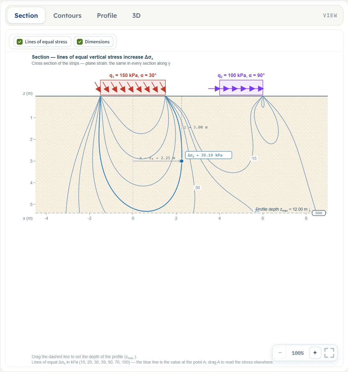
- Section is the cross-section of the strips on the ground surface, the point A with its dimension lines, and the profile depth. After Analyze it adds the lines of equal vertical stress increase and the value at A.
- Contours is the same cross-section coloured by the stress, on a logarithmic scale, with a legend in kPa and in per cent of q.
- Profile is the stress increase against depth under A: the total, the part from qv and the part from qh. Before Analyze it says “The profile appears after Analyze.”
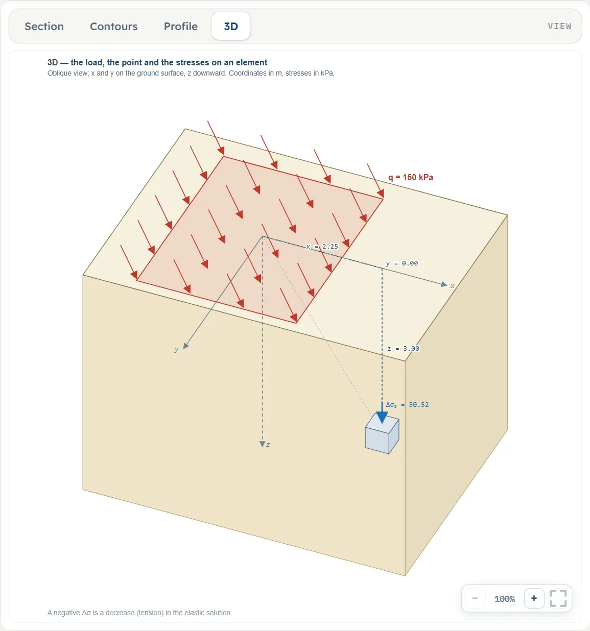
- 3D is an oblique block with the loaded strip, the axes x, y, z, the point A and the stress on a small element at A. Before Analyze it says “The stresses on the element appear after Analyze.”
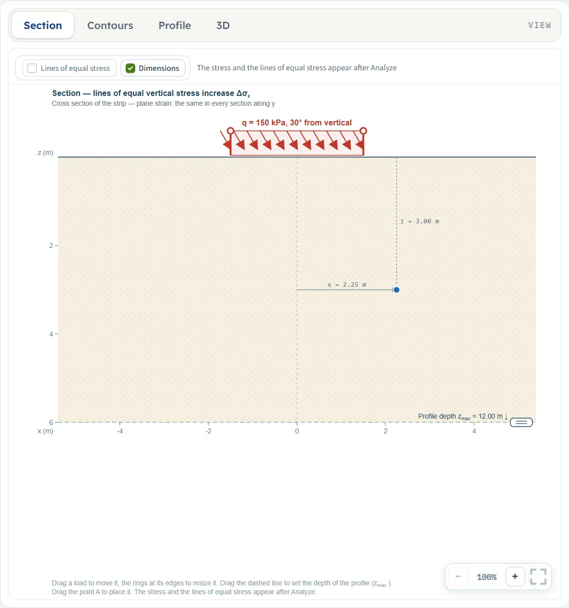
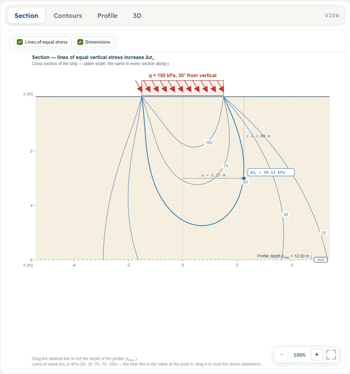
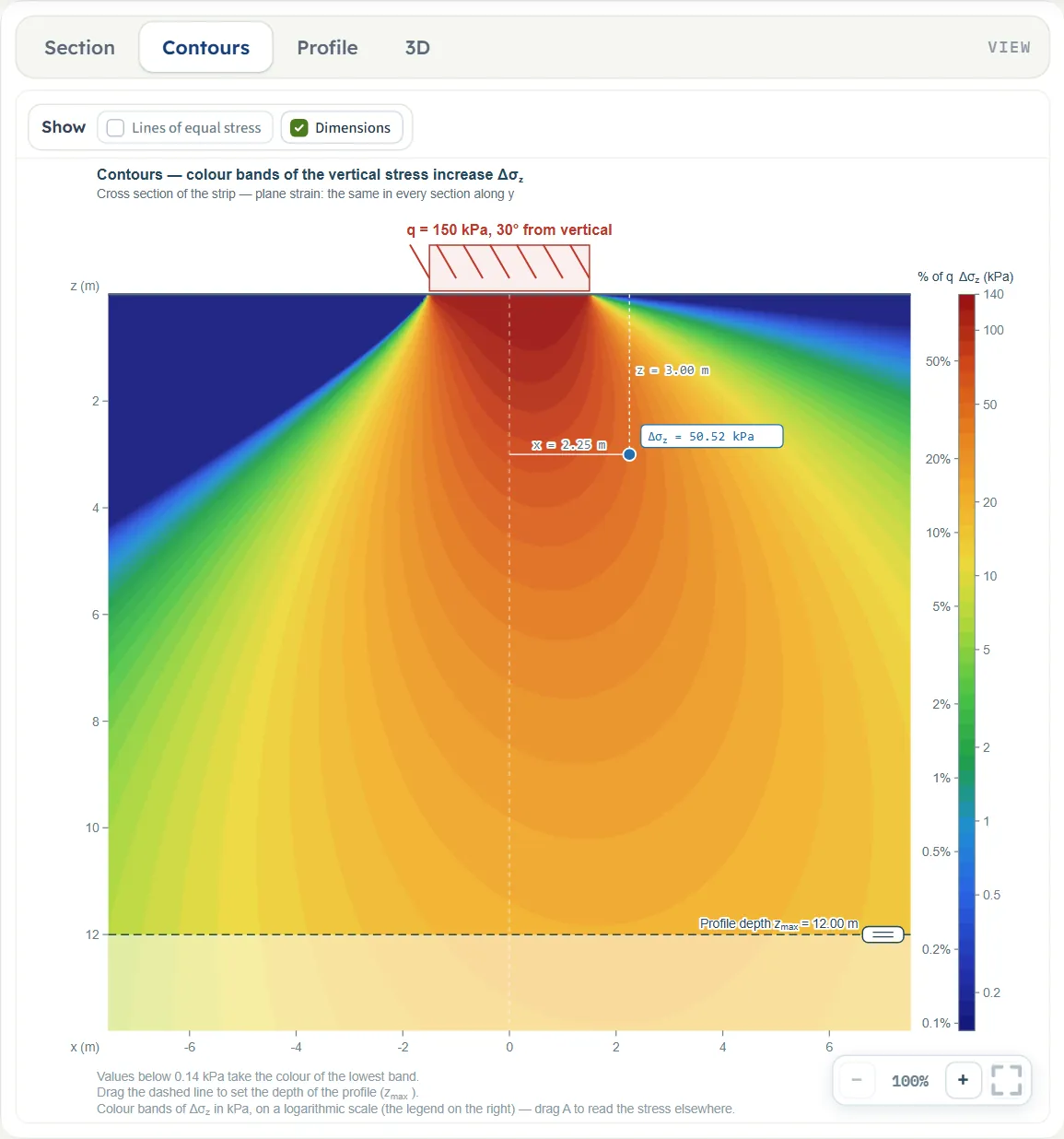
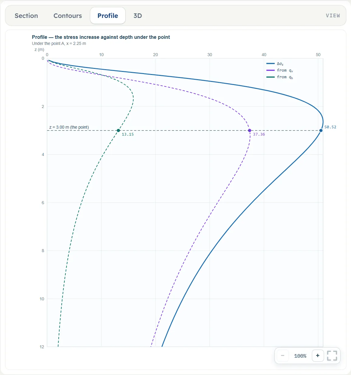
The Show chips
Above the Section and the Contours drawings a bar of two chips switches parts of the drawing on and off: Lines of equal stress and Dimensions. In the Section view both are on after Analyze; before it the lines are off and the bar says “The stress and the lines of equal stress appear after Analyze”. In the Contours view the lines are off by default (switch them on to draw them over the colours) and the bar says “The colour contours of the stress appear after Analyze”. The Profile and 3D views have no chips.
Dragging on the drawing
The drawing is a way of entering the model, and the Model tab follows every pull:
- A strip (Section, Contours and 3D, before Analyze). Drag the body of the strip along the ground to move its centre line xc. The same pulls work in the 3D view.
- The rings at the edges (before Analyze). Drag a ring to move that edge: the other edge stays, so B and xc change together. A pull cannot make a strip narrower than 0.1 m.
- The point A (Section and Contours, before and after Analyze). Drag A to move x and z. It stays inside the frame of the drawing, and its depth is at least 0.05 m. After Analyze the stress at A is recalculated at once and the Results tab follows.
- The dashed profile line (Section and Contours, before and after Analyze). Drag it up or down to set zmax; a pull cannot go above 0.5 m. When zmax is deeper than the drawing, the line sits at the lower edge with an arrow.
Pulls move in steps of 5 cm. A pull of a strip stops at the last free place, and the module says so (see Messages); two strips may meet at an edge but not overlap. After Analyze the strips and their rings are locked, together with every input of the model: Edit inputs unlocks them and clears the results. Only A and the profile line stay free.
Zoom and pan
Each view has −, a percentage and + at the lower right, and a button that fits the whole drawing in the pane. The mouse wheel zooms as well, and dragging the background moves the view.
Entering the model, section by section
The Model tab has four sections: Model data (names, files and quick saves, the same in every module), Strip loads, Point A and Depth profile. Each opens when you click its title; Next and Back at the foot walk you through Strip loads, Point A and Depth profile, and Analyze waits in the bar at the foot of the tab. The tables list every field with its symbol, the unit in each unit system and its default. Where a unit is shown twice or three times, such as m · ft, the units are those of SI · kN, SI · tf and US in turn, and equal ones are merged. Defaults are shown in SI; after a switch to US the boxes show the converted values, for example 3.13282 ksf for the 150 kPa strip, 9.84252 ft for the 3 m width and 7.38189 ft for x = 2.25 m.
Model data
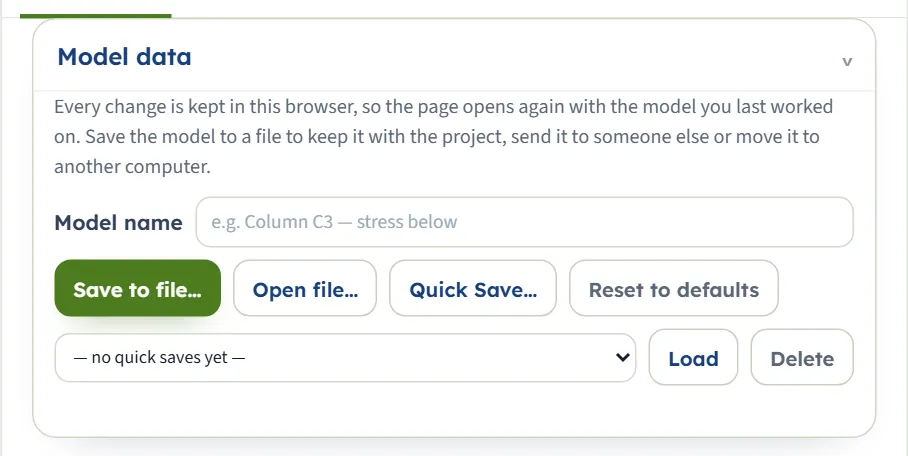
The first section holds the model name, Save to file…, Open file…, Quick Save… with its list and Load and Delete, and Reset to defaults. It works as described in the workspace guide. Reset returns the example at once and keeps it as the model of the browser.
Strip loads
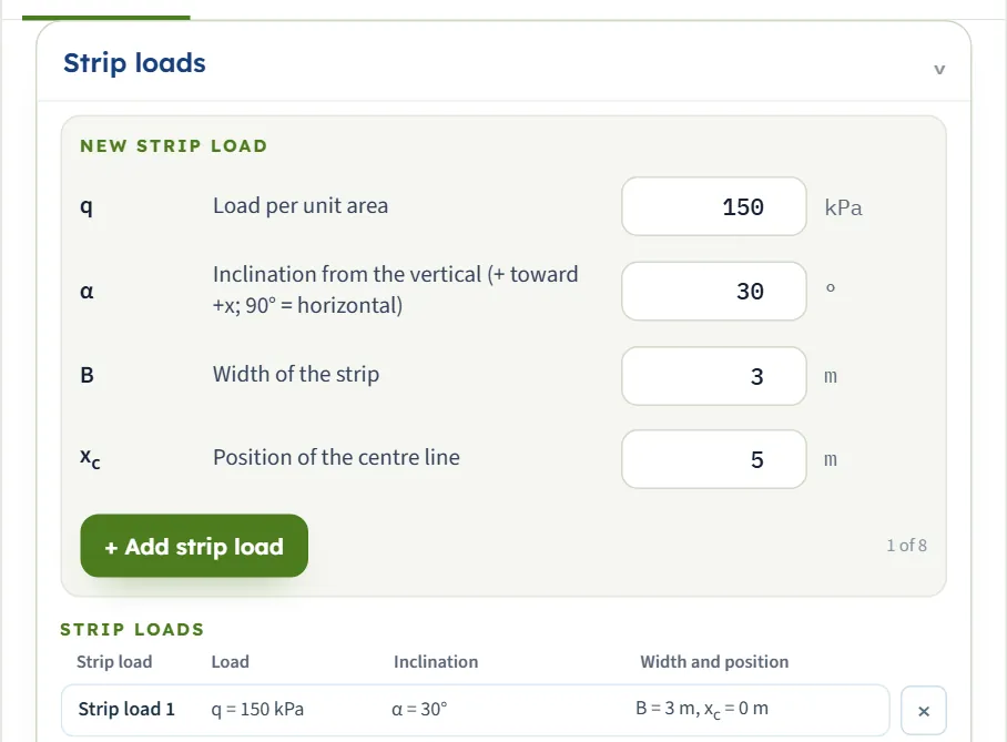
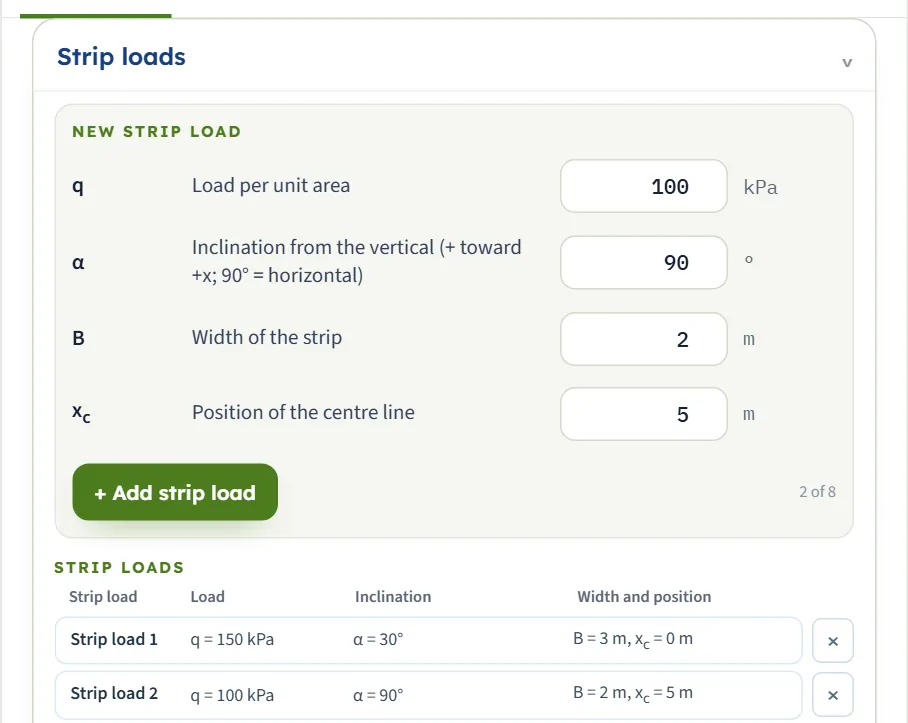
The section is a form over a table. The New strip load form takes the load q, the inclination α, the width B and the position xc of one strip. + Add strip load puts it at the bottom of the table, and a counter beside the button shows how many of the eight strips there are (1 of 8). The Strip loads table lists every strip as “q = 150 kPa”, “α = 30°” and “B = 3 m, xc = 0 m”. Press a row to change that strip in the form (the form then reads Editing · Strip load 1 and offers Done and Delete strip load; the note says that changes apply as they are entered), or press × to take a strip out. The stresses of the strips add.
| Field, unit and what to enter | Default |
|---|---|
| Load per unit area q Unit: kPa · t/m² · ksf Zero or more. This is the whole pressure, acting at the angle α; the module splits it into qv = q cos α and qh = q sin α. | 150 |
| Inclination from the vertical (+ toward +x; 90° = horizontal) α Unit: ° From −90° to 90°. 0° is a vertical load, 90° a horizontal load pushing toward +x, and a negative angle pushes toward −x. | 30 |
| Width of the strip B Unit: m · ft At least 0.001 m. | 3 |
| Position of the centre line xc Unit: m · ft Any value, along the same axis as the point A. Strip 1 is at 0; the New strip load form offers 5 m, so that a new strip does not lie on the first. | 0 · 5 (form) |
Two strips may meet at an edge but not overlap. The module checks this when you add a strip, when you change a value, and when you pull a strip on the drawing, and keeps the previous value if the change would put one strip on another (see Messages). After the eighth strip the button is off.
Point A
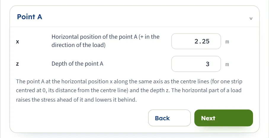
Two numbers place the point where you want the stress. With one strip at xc = 0, x is the distance from its centre line; with several strips it is the position on the common axis, and the dimension line on the drawing is the distance from the centre line of strip 1 (x − x₁). The note under the fields says that the horizontal part of a load raises the stress ahead of it and lowers it behind. A can also be dragged on the drawing.
| Field, unit and what to enter | Default |
|---|---|
| Horizontal position of the point A (+ in the direction of the load) x Unit: m · ft Any value. The axis does not turn with α: it is the axis of the centre lines, and + is the side toward which a load with a positive α pushes. | 2.25 |
| Depth of the point A z Unit: m · ft At least 0.001 m. The solution gives the stress inside the ground, so A cannot be on the surface. | 3 |
Depth profile
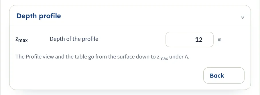
One number: how deep the table and the Profile view go under A. The table runs from the surface to zmax in ten equal steps (to the depth of A instead, if A is deeper than zmax) and the row of A is added; the Profile view shows at least zmax, and extends to 1.2 times the depth of A if A is deeper. The profile line on the Section and Contours drawings can be dragged to set it.
| Field, unit and what to enter | Default |
|---|---|
| Depth of the profile zmax Unit: m · ft At least 0.1 m. The table runs from the surface to zmax in ten equal steps (to the depth of A instead, if A is deeper than zmax) and the row of A is added; the Profile view shows at least zmax, and extends to 1.2 times the depth of A if A is deeper. | 12 |
Describing the load: inclination, direction and several strips
Three decisions shape the answer: the inclination of each strip, which side of the strip the point lies on, and how many strips there are.
| Inclination and what it is | kPa at x = 2.25 m |
|---|---|
| α = 0° A vertical strip: qh = 0. | 43.14, all vertical |
| α = 30° (default) Inclined; the horizontal part pushes toward +x. | 50.52 = 37.36 + 13.15 |
| α = 90° A horizontal strip pushing toward +x: qv = 0. | 26.31, all horizontal |
| α = −30° Inclined toward −x. | 24.21 = 37.36 + (−13.15) |
| α = −90° A horizontal strip pushing toward −x. | −26.31, a decrease |
Ahead of the load and behind it
The vertical part Δσz(v) is even in x: it is the same on both sides of the centre line. The horizontal part is odd in x: ahead of the load (the side toward which it pushes) the soil is pressed down, behind it the soil is lifted. In the example, A at +2.25 m gives 50.52 kPa (37.36 + 13.15) and A at −2.25 m gives 24.21 kPa (37.36 + (−13.15)); on the centre line, x = 0, the horizontal part is 0 and the total is 71.42 kPa. A negative angle α at x gives the mirror image of a positive angle at −x: the −30° strip at +2.25 m and the 30° strip at −2.25 m both give 24.21 kPa.
Several strips
Add a strip with its own q, α, B and xc. The module finds each strip’s stress with the distance of A from that strip’s centre line and adds them. In the Results tab the stress is “from the vertical parts” and “from the horizontal parts” of all strips, and, for two or three strips, a card gives the part of each strip.
With strip 2 added (100 kPa at 90°, 3 m wide, centre line at 5 m) the example gives 33.98 kPa at A: strip 1 gives 50.52 kPa and strip 2 −16.54 kPa, because A lies behind a strip that pushes away from it. With the point A at x = 2.5 m the total is 28.18 kPa. A strip 2 that meets strip 1 at an edge (centre line at 3 m, so that the edges touch at x = 1.5 m) gives 40.93 kPa. Four strips of the default kind at 0, 5, 10 and 15 m give 65.13 kPa at A, and eight strips at 0, 5 … 35 m give 64.82 kPa.
How to choose
- α follows the load. Use 90° for a pure shear along the surface (friction, braking, thrust) and the angle of the resultant for a load that has both parts; a load pushing toward −x takes a negative angle, or place A on the other side.
- Mirror to check. Changing the sign of α changes only the sign of the horizontal part; changing the sign of x does the same.
- One axis for everything. Strips and A are placed on one axis; type xc of each strip and x of A on it.
Analyze and read the results
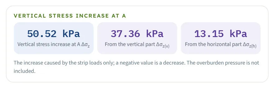
Press Analyze. The bar changes to Analysed — the stress at the point calculated and says “The inputs are locked. Edit inputs clears the results; the unit system can still be changed. The point A stays free: drag it on the drawing or change its coordinates, and the stress there is calculated at once.” The module stays on the Model tab: the value at A is written beside it on the drawing (Δσz = 50.52 kPa in the example), and the cards are in the Results tab.
| Card | Symbol | The example |
|---|---|---|
| Vertical stress increase at A | Δσz | 50.52 kPa |
| From the vertical part (“parts” for several strips) | Δσz(v) | 37.36 kPa |
| From the horizontal part (“parts” for several strips) | Δσz(h) | 13.15 kPa |
| From strip load 1, 2 … (two or three strips only) | Δσz(1) , Δσz(2) | strip 1 50.52, strip 2 −16.54 kPa in the two-strip case |
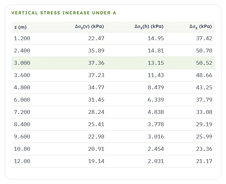
A note under the cards reads “The increase caused by the strip loads only; a negative value is a decrease. The overburden pressure is not included.” Below it, Values, step by step lists the vertical part, the horizontal part and their sum, and Vertical stress increase under A is a table that runs from the surface to zmax in ten equal steps (to the depth of A instead, if A is deeper than zmax) with the row of A added and marked, each with Δσz(v) , Δσz(h) and Δσz.
Using the numbers
- It is an increase. Add the overburden stress yourself where you need the total vertical stress; the module gives the change caused by the strips.
- Negative values are decreases (the elastic solution gives a lift behind a load that pushes away). The 3D view says “A negative Δσ is a decrease (tension) in the elastic solution.”
- The value at A and the profile follow the point as you drag it; the Results tab shows the stress at the new position.
- Changing the unit system after Analyze re-states the cards and the report without a new run; the drawings keep m and kPa when you change the unit system, while the boxes, cards, tables and report follow it. Edit inputs unlocks the model and clears the results.
Warnings
The bar carries a Warnings (0) button; it opens a window that says “No warnings — the assumptions of the solution hold for these inputs.”
The Calculations tab, the report and the Theory tab
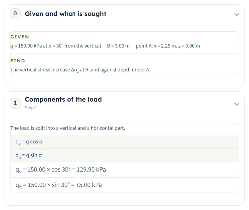
The Calculations tab opens with Given and what is sought and then writes out the working in numbered steps, ending with the answer. For one strip the steps are:
- Components of the load — qv = q cos α and qh = q sin α with your numbers: 129.90 kPa and 75.00 kPa in the example.
- Stress from the vertical part — the ratios 2x/B = 1.5000 and 2z/B = 2.0000, the strip factor Δσz/qv = 0.2876 and Δσz(v) = 0.2876 × 129.90 = 37.36 kPa.
- Stress from the horizontal part — the formula with b, x/b, z/b and x² + z² − b² = 11.8125, the factor 0.1754 and Δσz(h) = 0.1754 × 75.00 = 13.15 kPa.
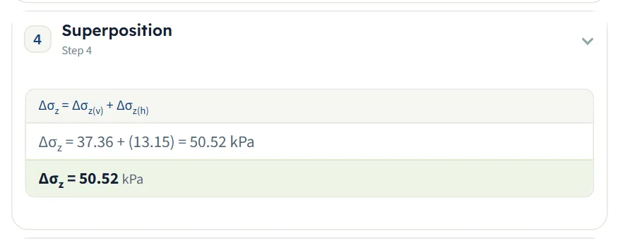
- Superposition — Δσz = Δσz(v) + Δσz(h) = 37.36 + (13.15) = 50.52 kPa.
- Stress increase against depth — the same sum down the vertical line through A, as a table with the row of A marked.
With several strips the working has one step for each strip (“Stress from strip load 1”, “… 2”, …), each with its own x, qv, qh and ratios, then the superposition of the strips and the depth table. The numbered steps are followed by an unnumbered Answer line.
The report
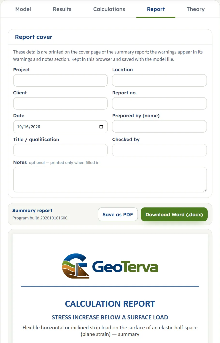
In the Report tab fill in the cover (project, location, client, report number, date, prepared by, title or qualification, checked by, and optional notes). The details are kept in this browser and saved with the model file. Save as PDF and Download Word (.docx) produce the summary report; the preview below the buttons is the report itself. Before Analyze the tab says “Press Analyze on the Model tab to calculate the stress at the point.”
The report has six parts: 1 Introduction and scope, 2 Input data, 3 Calculation (one part for each step of the Calculations tab), 4 Results, 5 Summary and 6 References. It carries the section with the lines of equal stress, the profile and the 3D view, and states the units used.
The Theory tab
The Theory tab has four sections: Scope and assumptions, The vertical stress, Worked examples and References. Each opens when you click its title, with Open all and Close all above them. It gives the formula for the horizontal strip, the chart of Δσz/q against x/b at several depths, a table of Δσz/q against z/b and x/b, and two worked examples whose numbers come from the module’s own code.
Worked example: the module’s own example
The module opens on this example, so you can follow the numbers on your own screen.
| Section | Input | Value |
|---|---|---|
| Strip loads | Strip load 1 | q = 150 kPa; α = 30°; B = 3 m; xc = 0 |
| Point A | Position and depth | x = 2.25 m; z = 3 m |
| Depth profile | Depth of the profile | zmax = 12 m |
Step 1: the two parts of the load
qv = 150 cos 30° = 129.90 kPa and qh = 150 sin 30° = 75.00 kPa. With B = 3 m, b = 1.5 m.
Step 2: the vertical part
The strip subtends ω = arctan(3.75/3) − arctan(0.75/3) = 51.34° − 14.04° = 37.30°, and δ = 14.04°. In radians ω = 0.6511; sin 37.30° = 0.6061 and cos(ω + 2δ) = cos 65.37° = 0.4168, so the factor Δσz/qv is (0.6511 + 0.6061 × 0.4168)/π = (0.6511 + 0.2526)/π = 0.2876, the value the Calculations tab gives, and Δσz(v) = 0.2876 × 129.90 = 37.36 kPa.
Step 3: the horizontal part
x² + z² − b² = 5.0625 + 9 − 2.25 = 11.8125, so the numerator is 4 × 1.5 × 2.25 × 9 = 121.5 and the denominator π(11.8125² + 4 × 2.25 × 9) = π × 220.54 = 692.8. The factor is 121.5 / 692.8 = 0.1754, and Δσz(h) = 0.1754 × 75.00 = 13.15 kPa.
Step 4: the sum
These are the three cards of the Results tab and the steps of the Calculations tab. The Profile view and the depth table give the same stress at the other depths: 50.52 kPa at 3 m, and 50.70 kPa at 2.4 m, 37.79 kPa at 6 m and 21.17 kPa at 12 m.
The point on the other side
Type x = −2.25 m: the vertical part is the same and the horizontal part changes sign, so Δσz = 37.36 − 13.15 = 24.21 kPa.
A purely horizontal strip
For q = 100 kPa, α = 90°, B = 4 m, x = 1 m and z = 1 m, b = 2 and Δσz = 4 × 2 × 100 × 1 × 1² / {π[(1 + 1 − 4)² + 4 × 4 × 1]} = 800 / (π × 20) = 12.73 kPa. The module gives 12.73 kPa, all from the horizontal part.
Other unit systems
The default example in SI · tf gives Δσz = 5.151 t/m² (3.810 + 1.341), and in US 1.055 ksf (0.7803 + 0.2747): the same strip in other units (50.52 kPa is 5.151 t/m² and 1.055 ksf). Two checks by hand:
- US. A horizontal strip of 2 ksf, B = 10 ft, x = 5 ft, z = 10 ft: b = 5 ft and Δσz = 4 × 5 × 2 × 5 × 10² / {π[(25 + 100 − 25)² + 4 × 25 × 100]} = 20 000 / (π × 20 000) = 0.3183 ksf. The module gives 0.3183 ksf.
- SI · tf. A strip of 10 t/m² at 60° from the vertical, B = 4 m, centre line at 1 m, A at x = 3 m and z = 2 m, so that the distance from the centre line is 2 m: qh = 8.660 and the horizontal part is 4 × 2 × 8.660 × 2 × 2² / {π[(4 + 4 − 4)² + 4 × 4 × 4]} = 554.3 / (π × 80) = 2.205 t/m². The module gives 2.205 t/m² for the horizontal part, 2.399 t/m² for the vertical part and 4.604 t/m² in all.
How each input changes the answer
Each row changes one thing in the example (strip 1: q = 150 kPa, α = 30°, B = 3 m, xc = 0; A at x = 2.25 m, z = 3 m) and runs the module again. The numbers are the ones the module gives, so you can reproduce any row. All values are in kPa; each was also found with an independent calculation. The last column gives the part from the vertical load qv plus the part from the horizontal load qh.
| Change | Δσz | qv + qh parts |
|---|---|---|
| The default example: q = 150 kPa, α = 30°, B = 3 m, xc = 0; A at x = 2.25 m, z = 3 m The reference | 50.52 | 37.36 + 13.15 |
| α = 0° A vertical strip: the horizontal part is zero | 43.14 | 43.14 + 0 |
| α = 60° A larger horizontal part and a smaller vertical part | 44.35 | 21.57 + 22.78 |
| α = 90° A horizontal strip: the vertical part is zero | 26.31 | 0 + 26.31 |
| α = −30° The horizontal part changes sign: A is now behind the load | 24.21 | 37.36 + (−13.15) |
| α = −90° A horizontal load pushing away from A: a decrease | −26.31 | 0 + (−26.31) |
| q = 300 kPa Twice the load, twice the stress | 101.0 | 74.73 + 26.31 |
| q = 0 No load, no stress | 0 | 0 + 0 |
| B = 6 m A wider strip: A is now under it (edge at x = 3 m) | 97.75 | 81.16 + 16.59 |
| B = 1.5 m A narrower strip | 24.60 | 17.44 + 7.162 |
| xc = 1.5 m The strip moved toward A (A is 0.75 m from the centre line) | 73.51 | 66.32 + 7.190 |
| x = 0 On the centre line the horizontal part is zero | 71.42 | 71.42 + 0 |
| x = −2.25 m The mirror point: the same vertical part, the opposite horizontal part | 24.21 | 37.36 + (−13.15) |
| x = 6 m Beyond the strip, far from the load | 7.807 | 3.754 + 4.053 |
| z = 0.5 m Near the surface | 12.09 | 5.165 + 6.929 |
| z = 1.5 m Shallower | 43.57 | 27.77 + 15.81 |
| z = 6 m Deeper | 37.79 | 31.45 + 6.339 |
| z = 12 m Deep: both parts fall off | 21.17 | 19.14 + 2.031 |
| Strip 2 added: q = 100 kPa, α = 90°, B = 3 m, xc = 5 m A lies behind strip 2, which lifts it (strip 1 gives 50.52, strip 2 −16.54) | 33.98 | 37.36 + (−3.384) |
| The same two strips, A at x = 2.5 m A moves 0.25 m nearer strip 2 | 28.18 | 32.48 + (−4.297) |
| Strip 2 with xc = 3 m (its edge meets that of strip 1) Strips that meet at an edge are allowed | 40.93 | 37.36 + 3.566 |
The pattern follows the formulas. The stress is proportional to q; the vertical part follows how much of the strip is seen from A; the horizontal part changes sign with α and with x and is zero on the centre line; and the stress of several strips is the sum of the single-strip stresses. The total under A is not largest at the surface: in the example it is 50.70 kPa at 2.4 m and 50.52 kPa at 3 m, and it falls to 21.17 kPa at 12 m.
Messages: when the module stops, and what it notes
The module checks the numbers it needs before it calculates. When one cannot be used it stops, and nothing is calculated.
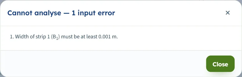
- If you press Analyze, a window titled Cannot analyse — 1 input error (or 2 input errors …) lists each message, and the box of the value is marked in its section of the Model tab (the section does not open by itself; open it to find the box).
- The limits are shown in the units of the unit system chosen.
| Stop when … | Message and what to do |
|---|---|
| The width is below 0.001 m or empty | “Width of strip 1 (B1) must be at least 0.001 m.” or “… is missing.” Enter a width. |
| The load is negative or empty | “Load per unit area of strip 1 (q1) must be at least 0 kPa.” or “… is missing.” Enter zero or a positive load; for a load that pushes the other way, use a negative inclination. |
| The inclination is outside −90° to 90° | “Inclination of the load of strip 1 from the vertical (+ toward +x; 90° = horizontal) (α1) must be at most 90°.” or “… at least -90°.” Enter an angle in that range. |
| The centre line is empty | “Position of the centre line of strip 1 (x1) is missing.” Enter the position. |
| The depth of A is below 0.001 m or empty | “Depth of the point A (z) must be at least 0.001 m.” or “… is missing.” Enter a depth below the surface. |
| The horizontal position of A is empty | “Horizontal position of the point A (+ in the direction of the load) (x) is missing.” |
| The depth of the profile is below 0.1 m | “Depth of the profile (zmax) must be at least 0.1 m.” |
When more than one value is wrong the window lists them together, for example “2 input errors”: “Width of strip 1 (B1) must be at least 0.001 m.” and “Depth of the point A (z) must be at least 0.001 m.” In the messages the strip number is part of the symbol: B1, q1, α1 and x1 belong to strip 1, B2 to strip 2.
Messages about overlapping strips
- Adding a strip on top of another: “The new strip load would lie on strip load 1 — they cannot overlap. Give it another position or width.”
- Changing a value that would put two strips on one another: “That would put strip load 1 and strip load 2 on top of one another — the value is kept as it was.”
- Pulling a strip on the drawing into another: the same message appears and the strip stays at the last free place, with its edge against the edge of the other (in the example, strip 1 pulled toward a strip at 5 m stops with its centre line at 2 m).
Notes and warnings
With usual values the Warnings window reads “No warnings — the assumptions of the solution hold for these inputs.” A negative result is not a warning: it is a decrease in the vertical stress, and the Results tab says so under the cards.
Good practice and common mistakes
- Choose α from the direction of the pressure. Zero is vertical and 90° horizontal; the sign sets which way the horizontal part pushes along x.
- Keep one axis. Type the centre lines xc and the point x on the same axis. The distance that matters is x − xc.
- Mind which side A is on. Ahead of a load that pushes toward +x the horizontal part adds to the stress; behind it, it subtracts. Run A on both sides when the point is near a loaded strip.
- Enter the pressure, not its vertical part. q is the whole pressure at the angle α; the module takes the vertical and horizontal parts itself.
- Strips may meet but not overlap. Split a strip of unequal loading into strips side by side.
- Add the overburden yourself. The module gives the increase caused by the strips.
- Read the profile as well as the point. The stress under A does not peak at the surface; the profile shows the depth at which it does (in the example near 2.4 to 3 m).
- Check the units after switching the system: type values in the units shown beside the boxes.
- Keep a record. The report is the record of an analysis; use Quick Save… or Save to file… to keep the model.
Frequently asked questions
How is the vertical stress below a horizontal strip load calculated?
The load q at the angle α from the vertical is split into qv = q cos α and qh = q sin α. The vertical part gives the stress of a vertical strip; the horizontal part gives Δσz(h) = 4bqhxz² / {π[(x² + z² − b²)² + 4b²z²]} with b = B/2; the two add. For the module’s example, Δσz = 50.52 kPa at A, of which 37.36 kPa is from the vertical part and 13.15 kPa from the horizontal part.
What is the difference between this module and Vertical strip load?
Vertical strip load takes loads that are purely vertical. This module takes a horizontal or inclined load, and with α = 0° it is a vertical strip too (the horizontal part is then zero). The vertical part of an inclined strip is found as for a vertical strip.
Which way are α and x positive?
α is measured from the vertical and is positive toward +x, so 90° is a horizontal load pushing toward +x and a negative angle pushes toward −x. x is measured along the axis of the centre lines, and does not turn with α. A strip at −30° read at +2.25 m gives the same stress as a strip at +30° read at −2.25 m (24.21 kPa in the example).
Why is the stress negative at some points?
The horizontal part is odd in x: the soil ahead of a load that pushes along the surface is pressed down, and the soil behind it is lifted, so Δσz is a decrease there. A horizontal strip of 150 kPa at α = −90° gives −26.31 kPa at the example point. A negative value is a decrease, not an error; the module does not call it a warning.
Why is the stress zero under the centre line for a horizontal strip?
The horizontal part is zero at x = 0 (0 kPa at 3 m in the example) because it is odd in x. A purely horizontal strip therefore adds no vertical stress under its centre line; an inclined strip still has the vertical part there (71.42 kPa at x = 0 in the example).
How many strips can I enter, and can they overlap?
Up to eight, each with its own q, α, B and centre line. They may meet at an edge but not overlap; the module keeps the previous value (or stops the pull) when a change would put one strip on another. The stresses of the strips add.
Can I drag the strips and the point A on the drawing?
Yes, before Analyze: drag a strip to move it, the rings at its edges to resize it, A to place the point, and the dashed line to set the profile depth. After Analyze the strips are locked until you press Edit inputs; A and the profile line stay free, and the stress at A is recalculated as you move it.
Does the stress include the weight of the soil?
No. The module gives the vertical stress increase caused by the strip loads. Add the overburden stress where you need the total.
What values does the module accept?
The load zero or more, the inclination from −90° to 90°, the width at least 0.001 m, any centre line, the depth of A at least 0.001 m, any position of A, and the profile depth at least 0.1 m. Anything else stops the analysis with a message that names the value.
Which units does it use, and what are the units of the answer?
SI · kN, SI · tf or US, switchable in the header at any time, even after Analyze. The stress is in kPa, t/m² or ksf, and lengths in m or ft. The default example gives 50.52 kPa, 5.151 t/m² or 1.055 ksf.
What does the report contain?
A cover with your project details and the answer, then six parts: introduction and scope, input data, the calculation step by step, results, summary and references, with the section, the profile and the 3D view. It is saved as a PDF or a Word file once the model is analysed.
Does the module remember my inputs?
Yes. Every change is kept in the browser, and the page opens again on the model you last worked on; an analysed model opens analysed only when nothing was changed after Analyze; if you moved or retyped A, or changed the profile depth, it opens with the new values and waits for Analyze. Reset to defaults brings back the example; Save to file and Quick Save keep copies.