

What the module calculates
At rest (K₀) gives the earth pressure at rest on a vertical wall that does not move: a basement wall braced by its floors, a bridge abutment on piles, a braced wall. The soil behind the wall keeps the state it had in the ground, so the horizontal effective stress is a fixed fraction K0 of the vertical effective stress, and the water adds its own pressure:
The force on the wall is the area of the pressure diagram, P0 = Ps + Pw, per unit length of wall, and the module also gives the height z̄ at which it acts above the base. For dry, uniform soil this reduces to P0 = ½ K0 γ H², acting at H/3 above the base.
What you can describe
- A wall of height H on level ground, with a water table behind it at any depth, or none.
- The backfill in up to six layers, from the top down. Each layer has its own unit weights and its own K0, found by one of four relationships: Jaky / Mayne–Kulhawy, Massarsch (clay), Sherif (compacted sand) or a value you give, Given K₀.
The module draws the section, the pressure on the wall and a 3D view, writes out the working step by step, and prepares a PDF or Word report.
What belongs to other modules
- This module is for a wall that does not move. A wall that yields enough for the soil to reach its active state is the case of the other modules of this family, starting with Rankine and Coulomb; a wall pushed into the soil is the passive case, in Passive, log spiral.
- The result is the pressure of the soil and the water. A load on the ground behind the wall is added from the Surcharge loads modules, for example Uniform load, and the combination is made in your wall calculation.
Before you start: what you need
Have these ready from your design:
| What | Notes |
|---|---|
| The wall height H From: Your design | From the top of the retained ground to the base of the wall; at least 0.1 m. |
| The soil layers behind the wall: thickness, γ and γsat From: Boring logs, laboratory tests | From the top down, up to six layers. The last layer runs on to the base of the wall, so it needs no thickness. |
| For each layer, what its K0 will come from From: Tests or correlations | φ′ and OCR for Jaky / Mayne–Kulhawy; PI and OCR for Massarsch (clay); φ′, γd and γd(min) for Sherif (compacted sand); or K0 itself. |
| Water table depth zw From: Piezometers, borings | Behind the wall only; there is no water in front of it. Optional: choose None for a dry backfill. |
Quick start in seven steps
- Open the module and choose the units
Open At rest (K₀) from the Lateral Earth Pressure family. Pick SI · kN, SI · tf or US in the header. Open At rest (K₀).
- Enter the wall
In Wall, type the height H.
- Describe the soil layers
In Soil layers, choose how K0 is found, fill in the thickness and the soil values, and press + Add layer. The example’s layer is already in the table; add more from the top down.
- Set the groundwater
In Groundwater, choose Present and give the depth zw, or None.
- Press Analyze
Press Analyze at the foot of the Model tab. The bar reads Analysed and the inputs lock. The module stays on the Model tab and the Section view: press Pressure above the drawing to see the pressure.
- Read the answer
The Results tab gives P0, its height z̄ above the base and the shares of the soil and the water, with K0 of every layer and the stresses at the breaks of the diagram.
- Take the working and the report
The Calculations tab shows the three steps with your numbers. The Report tab saves a PDF or a Word file.
The screen: three views of the wall
The layout is the one every GeoTerva module shares, described in the workspace guide. For this module the drawing has three views, chosen with the buttons above it:
- Section shows the wall, the soil layers with their properties and the water table, with the dimensions. It follows your inputs as you type; after Analyze each layer also carries its K0.
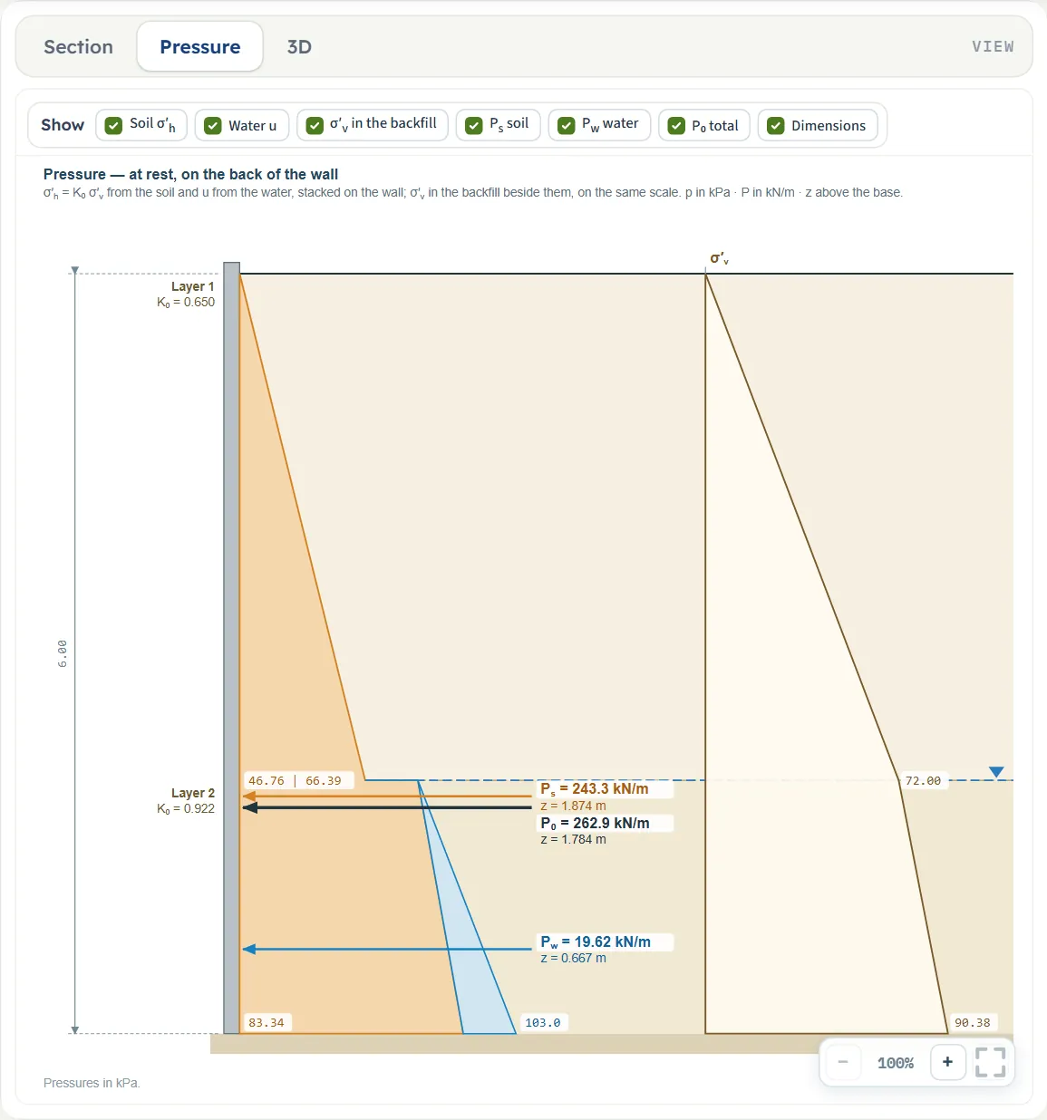
- Pressure shows the at-rest pressure on the back of the wall after Analyze: σ′h from the soil and u from the water, stacked, the resultants Ps, Pw and P0 with their heights above the base, and σ′v in the backfill beside them on the same scale. Before Analyze it shows the wall, the layers and the water table only.
- 3D shows a length of the wall with the backfill on its right; after Analyze it adds the pressure prism on the face of the wall, σ′h + u, and the resultant.
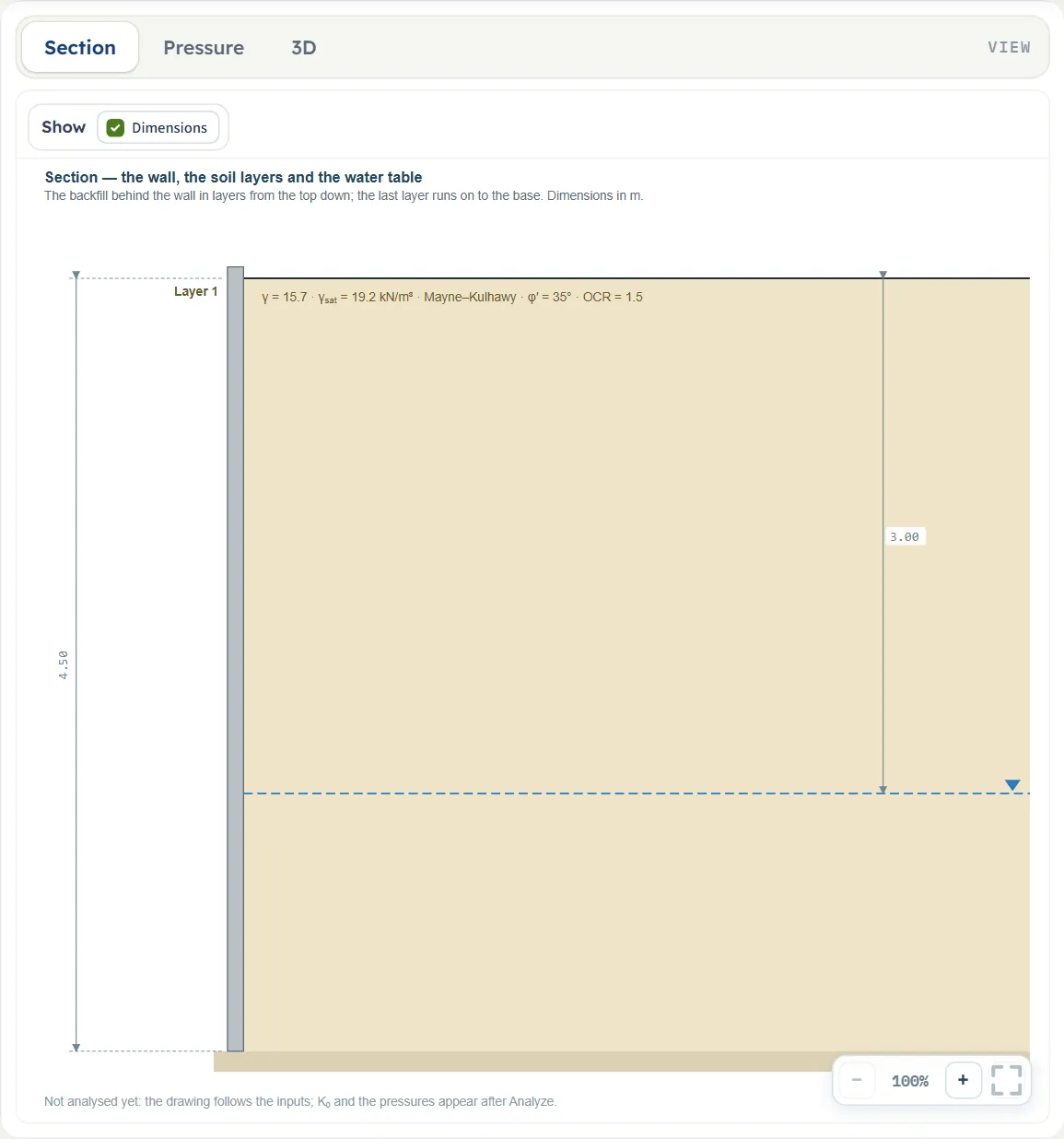
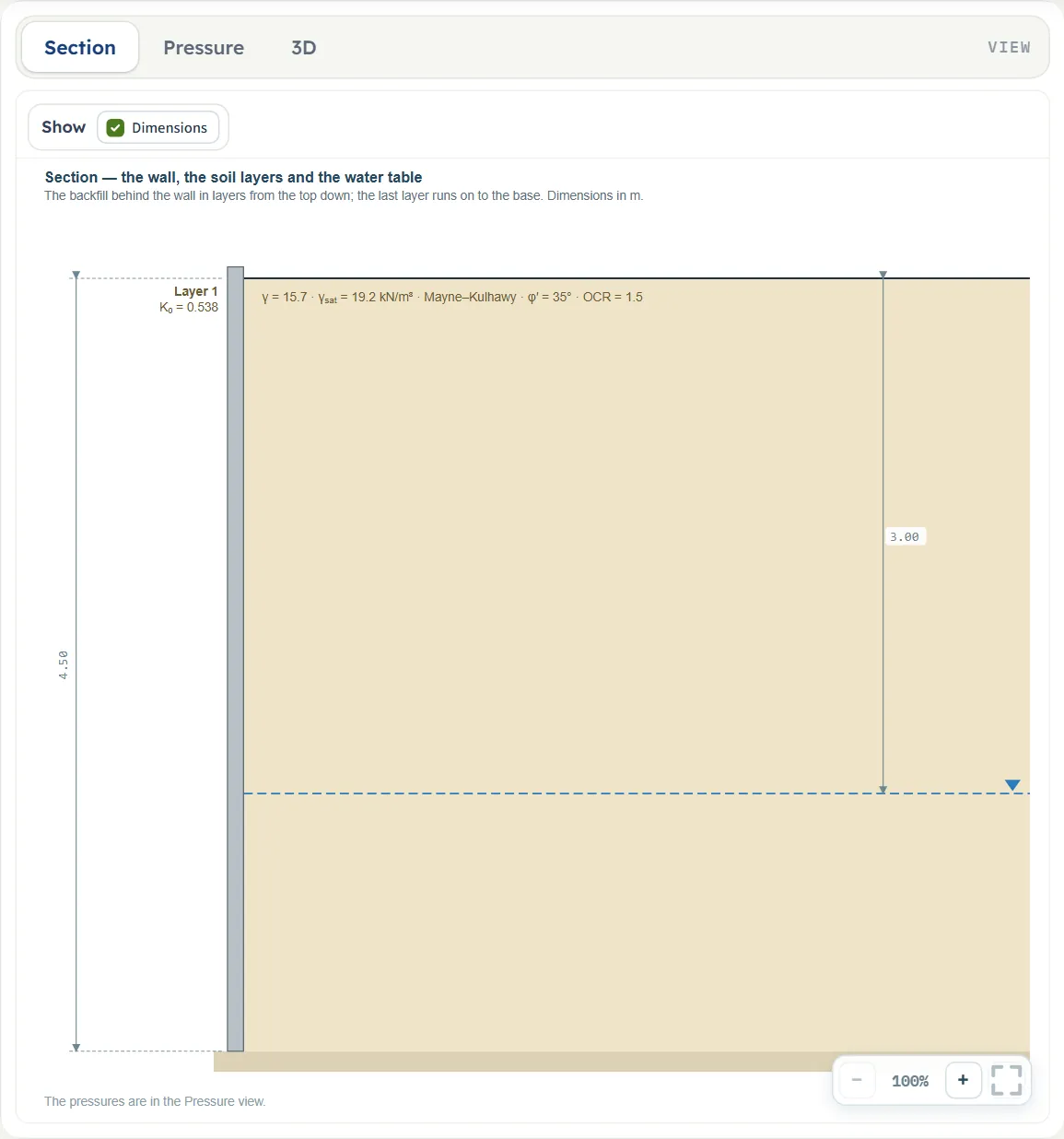
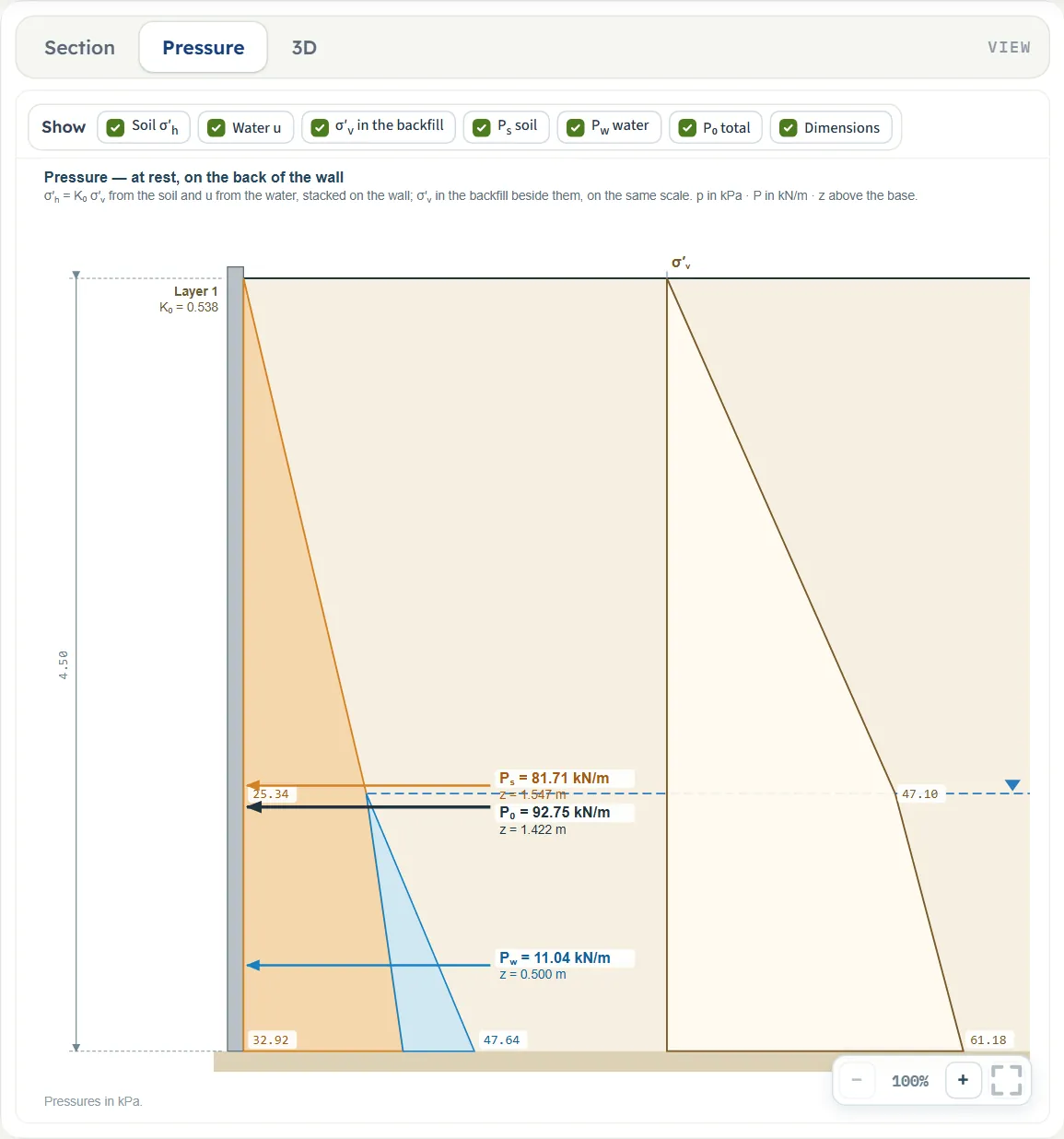
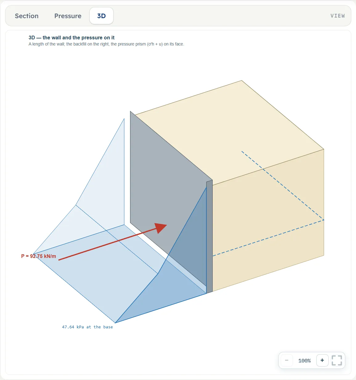
The Show chips
Above the drawing a Show bar switches parts of it on and off. In the Section view there is one chip, Dimensions. In the Pressure view there are seven: Soil σ′h, Water u, σ′v in the backfill, Ps soil, Pw water, P₀ total and Dimensions. Before Analyze the six result chips are unchecked and the bar says “The pressures and the resultant appear after Analyze”; after it they are all checked, and you can hide any of them, for example to read the water pressure alone. Dimensions shows or hides the height of the wall and the heights of the resultants. The 3D view has no chips.


Entering the model, section by section
The Model tab has Model data and three sections: Wall, Soil layers and Groundwater. Wall, Soil layers and Groundwater work as an accordion: opening one closes the other two. Model data opens and closes on its own. Next and Back at the foot walk you through them. The tables list each field with its symbol, the unit in each unit system and its default. Where a unit is shown twice or three times, such as m · ft, the units are those of SI · kN, SI · tf and US in turn, and equal ones are merged. Defaults are those of the example, in SI · kN; after a change of unit the boxes hold the converted values unrounded: in SI · tf the unit weights read 1.60095 and 1.95786 t/m³, and in US the boxes read 14.7638 ft for the wall, 99.9443 pcf, 122.225 pcf and 9.84252 ft (the water depth and the thickness) for the same wall and soil.
Model data
The first section is the one every module has: a Model name, Save to file… and Open file…, Quick Save… (it asks for a name and keeps that version in this browser, to be brought back with Load or removed with Delete) and Reset to defaults, which returns to the example at once. Every change you make is also kept in this browser as you work. If you close the page and open it again the model you last worked on is there, and an analysed model comes back analysed and locked. See the workspace guide.
Wall
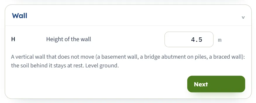
One number: the height of the wall. The note in the section says what the module assumes: a vertical wall that does not move, with level ground behind it.
| Field | Unit | Default |
|---|---|---|
| Height of the wall H From the top of the retained ground to the base of the wall. At least 0.1 m; an empty box stops the analysis. | m ft | 4.5 |
Soil layers
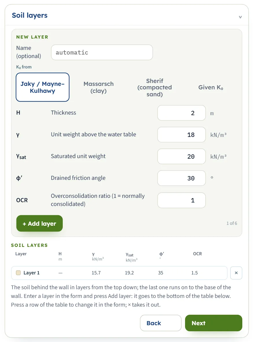
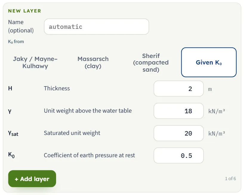
The layers are entered one at a time from the top down. The New layer form at the top holds the values of the layer you are about to add; the Soil layers table under it lists the layers already in the model, each with its own colour, as on the drawing.
- Choose how K0 of the layer is found with the four buttons under K₀ from. The boxes below the buttons follow the choice.
- Fill in the thickness and the soil values, and press + Add layer. The layer goes to the bottom of the table and the counter (“1 of 6”) moves on. The form keeps its values, so the next layer starts from them.
- To change a layer, press its row in the table: the layer opens in the form and changes apply as you type. The × at the end of a row takes the layer out.
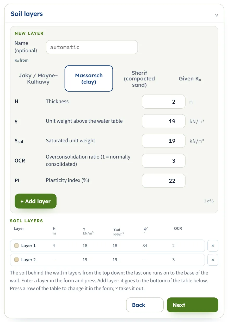
The table shows H, γ, γsat, φ′ and OCR of each layer; a dash stands where a layer has no such value, such as φ′ of a Massarsch layer. The values in the field table are those of the example’s layer; the form for a new layer opens at 2 m, 18 and 20 kN/m³, 30°, OCR 1, PI 20, γd 17, γd(min) 15 and K₀ 0.5.
| Field | Unit | Default |
|---|---|---|
| Name (optional) A name for the drawing and the tables; left empty, the layers are called Layer 1, Layer 2 and so on. | — | automatic |
| Thickness Hi At least 0.01 m. The thickness of the last layer is not used: it runs on to the base of the wall, and the table shows a dash for it. | m ft | 3 |
| Unit weight above the water table γ At least 1 kN/m³. | kN/m³ t/m³ pcf | 15.7 |
| Saturated unit weight γsat At least 1 kN/m³. Below the water table the module uses γsat − γw for the vertical effective stress. Shown when the water table is Present. | kN/m³ t/m³ pcf | 19.2 |
| Drained friction angle φ′ From 0° to 50°. Shown when K₀ from is Jaky / Mayne–Kulhawy or Sherif (compacted sand). | ° | 35 |
| Overconsolidation ratio (1 = normally consolidated) OCR At least 1. Shown when K₀ from is Jaky / Mayne–Kulhawy or Massarsch (clay). | — | 1.5 |
| Plasticity index (%) PI At least 0. Shown when K₀ from is Massarsch (clay). | — | 20 |
| Compacted dry unit weight behind the wall γd At least 1 kN/m³, and not below the next value. Shown when K₀ from is Sherif (compacted sand). | kN/m³ t/m³ pcf | 17 |
| Dry unit weight in the loosest state γd(min) At least 1 kN/m³. Shown when K₀ from is Sherif (compacted sand). | kN/m³ t/m³ pcf | 15 |
| Coefficient of earth pressure at rest K0 From 0 to 3. Shown when K₀ from is Given K₀. | — | 0.5 |
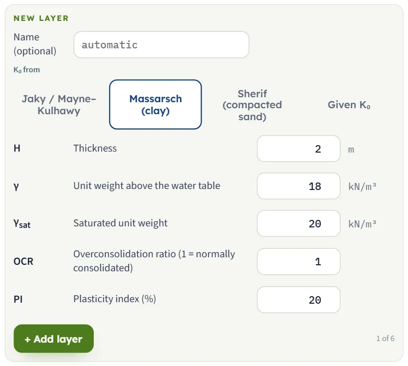
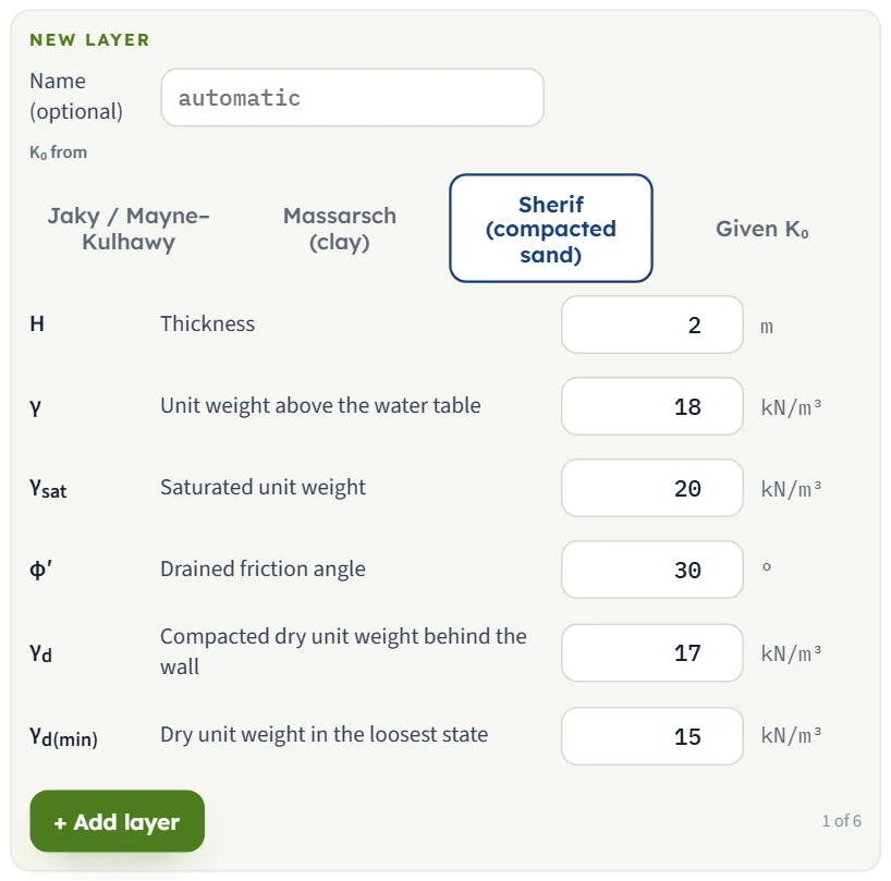
The boxes of the New layer form change with the relationship chosen. Massarsch (clay) asks for the overconsolidation ratio and the plasticity index and has no friction angle. Sherif (compacted sand) asks for φ′, the compacted dry unit weight γd and the loosest-state value γd(min), and has no OCR. Given K₀ asks for K0 alone.
Groundwater
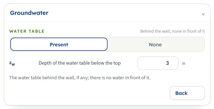
Choose Present or None. With a water table the depth zw is asked for, and the layers ask for their saturated unit weight. The water is behind the wall only: the module takes no water in front of it. A water table at the base of the wall or below it gives no water pressure on the wall.
| Field | Unit | Default |
|---|---|---|
| Depth of the water table below the top zw Zero or more. Shown when Water table is Present. | m ft | 3 |
Choosing how K₀ is found
K0 is the one decision of this module, and each layer has its own. The four relationships:
| Option | Coefficient |
|---|---|
| Jaky / Mayne–Kulhawy (the default) Use it for sand, gravel and other soils for which you hold φ′; the second form for overconsolidated soil, from clay to gravel. | K0 = 1 − sin φ′ (Jaky 1944) when OCR = 1; K0 = (1 − sin φ′) OCRsin φ′ (Mayne and Kulhawy 1982) when OCR is above 1 |
| Massarsch (clay) Use it for fine-grained soil for which you hold the plasticity index. With OCR = 1 the factor is 1. | K0 = [0.44 + 0.42 PI/100] √OCR (Massarsch 1979 for the normally consolidated value; × √OCR when overconsolidated) |
| Sherif (compacted sand) Use it for a compacted sand fill behind the wall, where compaction raises the pressure above Jaky’s value. | K0 = (1 − sin φ′) + 5.5 [γd/γd(min) − 1] (Sherif, Fang and Sherif 1984) |
| Given K₀ Use it for a value from a test or another source. | K0 from 0 to 3, as you enter it |
How they compare
The table gives K0 as the module returns it for the example’s layer (φ′ = 35°, γ = 15.7 kN/m³, water table at 3 m) with one relationship changed at a time, and the force P0 on the 4.5 m wall that follows.
| Relationship | K0 | P0 | z̄ |
|---|---|---|---|
| Jaky, OCR = 1 | 0.426 | 75.79 | 1.394 |
| Mayne–Kulhawy, OCR = 1.5 (the example) | 0.538 | 92.75 | 1.422 |
| Mayne–Kulhawy, OCR = 3 | 0.801 | 132.6 | 1.460 |
| Massarsch, PI = 20, OCR = 1.5 | 0.642 | 108.5 | 1.440 |
| Sherif, γd = 17, γd(min) = 15 kN/m³ | 1.160 | 187.2 | 1.485 |
| Given K0 = 0.5 | 0.500 | 86.97 | 1.414 |
Which should I pick?
- Start from what you know about the soil. A normally consolidated sand or gravel with a measured φ′: Jaky with OCR = 1. An overconsolidated soil: keep Jaky / Mayne–Kulhawy and enter the OCR.
- Use Massarsch for a clay when the plasticity index is what you hold.
- Use Sherif only for a compacted fill, with the unit weights it asks for. The module stops if the compacted unit weight is below the loosest-state value.
- Use Given K₀ for a value of your own. The module accepts 0 to 3 and, as for any layer, shows a caution above 3 (see the messages).
- Different layers, different relationships. A sand fill over a clay can use Jaky / Mayne–Kulhawy in the first layer and Massarsch in the second.
Analyze and read the results
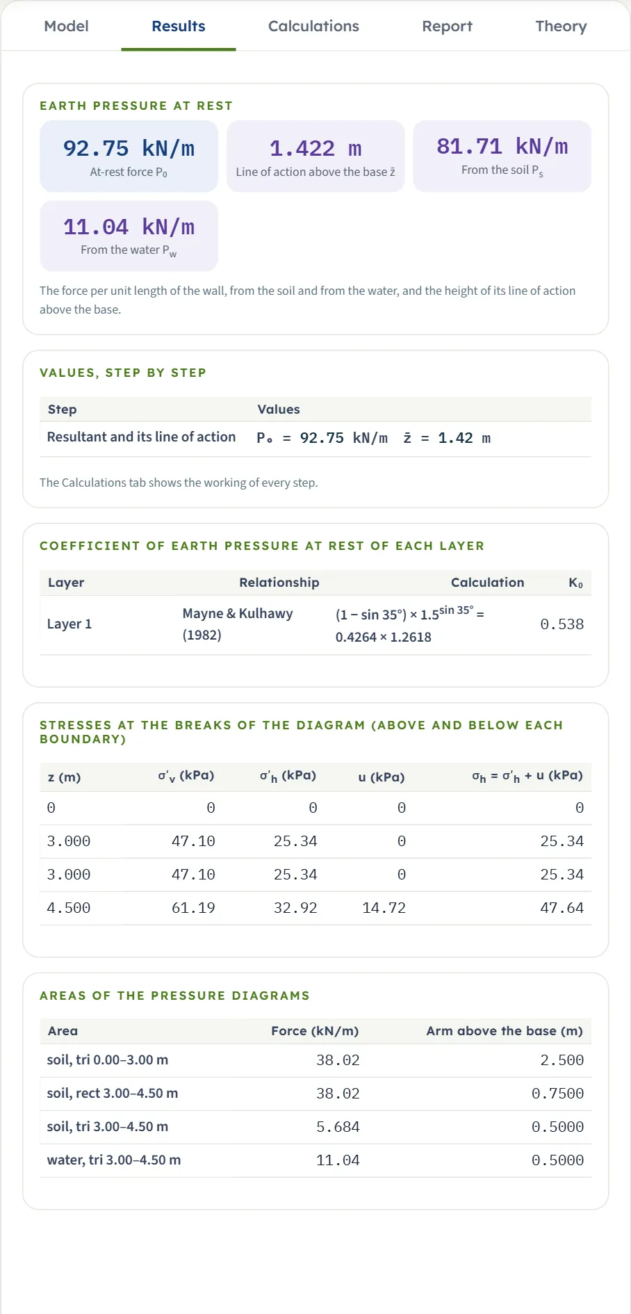
Press Analyze. The bar changes to Analysed — the earth pressure calculated and says “The inputs are locked. Edit inputs clears the results; the unit system can still be changed.” The Warnings button beside Edit inputs shows the number of cautions of the run. The Results tab then holds five blocks, and the Pressure view above the drawing carries the pressure. The drawings always read in m, kPa and kN/m; the cards, the tables and the report follow the unit system.
| Card | The example |
|---|---|
| At-rest force P0 The resultant of the soil and the water pressure per unit length of wall. | 92.75 kN/m |
| Line of action above the base z̄ The height of P0 above the base of the wall. | 1.422 m |
| From the soil Ps The area of the effective-pressure diagram. | 81.71 kN/m |
| From the water Pw The area of the pore-pressure diagram; zero for no water, or a water table at or below the base. | 11.04 kN/m |
Under the cards the tab lists: Values, step by step (the answer of the last step); Coefficient of earth pressure at rest of each layer (the relationship, its working and K0); Stresses at the breaks of the diagram, with σ′v, σ′h, u and σh = σ′h + u above and below each boundary and at the base; and Areas of the pressure diagrams, each with its force and its arm above the base.
Using the numbers
- P0 is a force per unit length of wall, in kN/m (tf/m or kip/ft in the other systems), acting at z̄ above the base. The soil and the water are separate parts: Pw acts at a third of the water’s height above the water’s own base.
- Changing the unit system after Analyze re-states the cards, the tables and the report without a new run. Edit inputs unlocks the model and clears the results.
- A load on the ground behind the wall is not in these numbers. Add it from the Surcharge loads modules in your wall calculation.
The Calculations tab, the report and the Theory tab
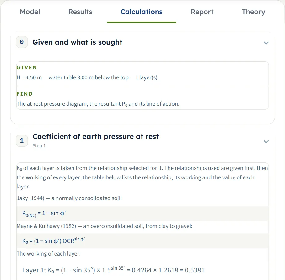
The Calculations tab writes out the working in numbered steps, after a Given and what is sought block:
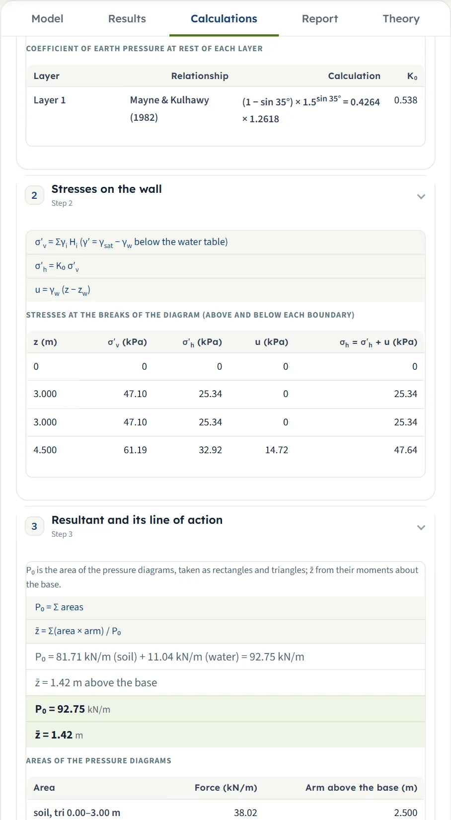
- Coefficient of earth pressure at rest. The relationships used are given first, then the working of every layer with its numbers, and a table of the relationship, the working and K0 of each layer.
- Stresses on the wall. σ′v = Σγi Hi (with γ′ = γsat − γw below the water table), σ′h = K0 σ′v and u = γw (z − zw), then the table of stresses at the breaks of the diagram.
- Resultant and its line of action. P0 is the sum of the areas, z̄ = Σ(area × arm) / P0, with the table of areas and the answer of each part.
The tab ends with an Answer line, for the example: P₀ = 92.75 kN/m, acting 1.42 m above the base. Before Analyze the tab asks you to analyse first.
The report
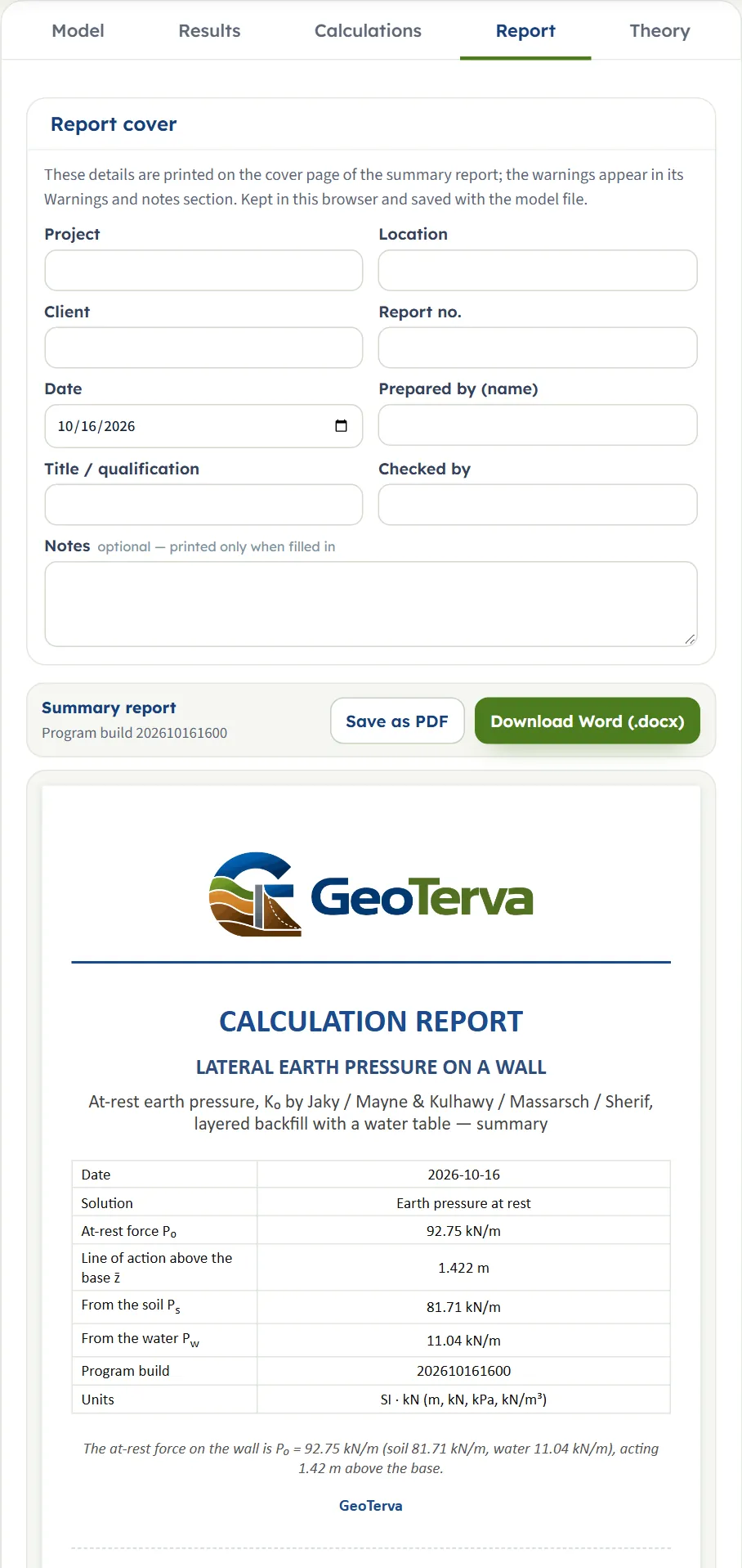
In the Report tab fill in the cover (project, location, client, report number, date, prepared by, title or qualification, checked by, and optional notes). The details are kept in this browser and saved with the model file. After Analyze, Save as PDF and Download Word (.docx) produce the report; the preview below the buttons is the report itself.
The report has six parts (seven when the run has cautions): 1 Introduction and scope, 2 Input data, 3 Calculation (3.1 the coefficient, 3.2 the stresses, 3.3 the resultant), 4 Results, 5 Summary and 6 References. It carries the section, the pressure and the 3D drawings and states the units with the conversion constants. When the run has cautions, a seventh part, Assumptions and notes, is added before the Summary and prints them.
The Theory tab
The Theory tab has six sections that open and close, with Open all and Close all: Earth pressure at rest; The coefficient K₀; Dry backfill; Partially submerged backfill; Worked examples (a wall in sand with a water table, and a wall in sand over clay); and References. The first worked example is the module’s own example.
Worked examples
The module opens on the first example, so you can follow its numbers on your own screen.
| Section | Input | Value |
|---|---|---|
| Wall | Height | H = 4.5 m |
| Soil layers | One layer, Jaky / Mayne–Kulhawy | γ = 15.7 kN/m³, γsat = 19.2 kN/m³, φ′ = 35°, OCR = 1.5 |
| Groundwater | Present | zw = 3 m |
Step 1: the coefficient
K0 = (1 − sin 35°) × 1.5sin 35° = 0.4264 × 1.2618 = 0.538.
Step 2: the stresses
At the water table, 3 m down: σ′v = 15.7 × 3 = 47.10 kPa and σ′h = 0.5381 × 47.10 = 25.34 kPa. At the base, with γ′ = 19.2 − 9.81 = 9.39 kN/m³: σ′v = 47.10 + 9.39 × 1.5 = 61.19 kPa (61.185 exactly: the tables show 61.19 and the drawing 61.18), σ′h = 32.92 kPa and u = 9.81 × 1.5 = 14.72 kPa, so σh = 47.64 kPa.
Step 3: the resultant
| Area | kN/m | Arm (m) |
|---|---|---|
| Soil, triangle 0–3 m: ½ × 3 × 25.34 | 38.02 | 2.500 |
| Soil, rectangle 3–4.5 m: 1.5 × 25.34 | 38.02 | 0.7500 |
| Soil, triangle 3–4.5 m: ½ × 1.5 × (32.92 − 25.34) | 5.684 | 0.5000 |
| Water, triangle 3–4.5 m: ½ × 1.5 × 14.72 | 11.04 | 0.5000 |
Ps = 38.02 + 38.02 + 5.684 = 81.71 kN/m, Pw = 11.04 kN/m, so P0 = 92.75 kN/m. The moments about the base give z̄ = (95.04 + 28.51 + 2.84 + 5.52) / 92.75 = 1.422 m. These are the four cards of the Results tab, and the three steps of the Calculations tab.
A second example: sand over clay
A 6 m wall retains 4 m of sand (γ = γsat = 18 kN/m³, φ′ = 34°, OCR = 2) over a clay (γ = γsat = 19 kN/m³, PI = 22, OCR = 3), with the water table at the top of the clay, 4 m down. Set H = 6 m and zw = 4 m, change layer 1 (thickness 4 m) in the table, and add the clay with Massarsch (clay).
K0 of the sand is (1 − sin 34°) × 2sin 34° = 0.4408 × 1.4734 = 0.650, and of the clay [0.44 + 0.42 × 22/100] × √3 = 0.5324 × 1.7321 = 0.922. At 4 m σ′v = 72.00 kPa, so σ′h is 46.76 kPa in the sand and 66.39 kPa in the clay: the diagram steps at the boundary. At 6 m, with γ′ = 19 − 9.81 = 9.19 kN/m³, σ′v = 72.00 + 18.38 = 90.38 kPa, σ′h = 83.34 kPa and u = 19.62 kPa. The areas are 93.53, 132.8 and 16.95 kN/m of soil and 19.62 kN/m of water.
The module gives Ps = 243.3 kN/m, Pw = 19.62 kN/m, P0 = 262.9 kN/m and z̄ = 1.784 m.
A check in US units and in SI · tf
Switch to US, enter a 15 ft wall with γ = 100 pcf, φ′ = 30°, OCR = 1 and no water. K0 = 1 − sin 30° = 0.5 and, by hand, P0 = ½ × 0.5 × 100 × 15² = 5625 lb/ft and z̄ = 15/3 = 5 ft. The module gives 5.625 kip/ft at 5.000 ft.
In SI · tf a 5 m wall with γ = 1.8 t/m³, φ′ = 30°, OCR = 1 and no water gives, by hand, ½ × 0.5 × 1.8 × 5² = 11.25 tf/m at 5/3 = 1.667 m; the module gives 11.25 tf/m at 1.667 m.
How each input changes the answer
Each row changes one thing in the example (4.5 m wall, one layer of φ′ = 35°, OCR = 1.5, γ = 15.7 and γsat = 19.2 kN/m³, water table at 3 m) and runs the module again. The numbers are the ones the module gives, so you can reproduce any row. Forces are in kN/m, heights in m above the base.
| Change | K0 | P0 | z̄ |
|---|---|---|---|
| The example The reference: Ps 81.71, Pw 11.04 | 0.538 | 92.75 | 1.422 |
| H = 6 m Both parts grow; the water table is still at 3 m | 0.538 | 180.9 | 1.840 |
| Water table None Dry soil: P0 = ½ K0 γ H², at H/3 | 0.538 | 85.53 | 1.500 |
| zw = 1.5 m More soil submerged: Pw 44.15 | 0.538 | 114.4 | 1.374 |
| zw = 0 The whole wall under water: Pw 99.33 | 0.538 | 150.5 | 1.500 |
| zw = 4.5 m No water pressure: the same as dry | 0.538 | 85.53 | 1.500 |
| φ′ = 30° A smaller φ′ raises K0 | 0.612 | 104.0 | 1.436 |
| φ′ = 40° A larger φ′ lowers K0 | 0.464 | 81.44 | 1.405 |
| OCR = 1 Jaky’s value, the smallest K0 here | 0.426 | 75.79 | 1.394 |
| OCR = 3 Overconsolidation raises K0 | 0.801 | 132.6 | 1.460 |
| γ = 18, γsat = 20 kN/m³ Heavier soil: Ps 93.34 | 0.538 | 104.4 | 1.440 |
| γsat = 21 kN/m³ Only the soil below the water table changes; Pw does not | 0.538 | 93.84 | 1.411 |
| Massarsch, PI = 20 A different relationship for the same layer | 0.642 | 108.5 | 1.440 |
| Sherif, 17 over 15 kN/m³ Compaction raises K0 above 1 | 1.160 | 187.2 | 1.485 |
| Given K0 = 1 Pressure as in a fluid of the soil’s weight | 1.000 | 162.9 | 1.476 |
| A second layer: φ′ = 30°, OCR = 1, below 3 m The diagram steps where K0 changes | 0.538 / 0.500 | 90.11 | 1.442 |
| A second layer: Massarsch, PI = 30, OCR = 2, γ = 18, γsat = 19 kN/m³, below 3 m A larger K0 in the lower layer | 0.538 / 0.800 | 113.9 | 1.292 |
The pattern follows the formulas. K0 is a property of each layer: it falls as φ′ grows and rises with the OCR. A higher water table adds water pressure, which does not depend on K0, and takes weight off the soil below it, so Ps falls while Pw grows. The height z̄ is H/3 for dry soil. With a water table inside the wall it sits a little below H/3 (1.37 to 1.42 m in these rows) because the water diagram is a triangle on the lower part of the wall; with the water at the surface the whole diagram is triangular again and z̄ returns to H/3 (1.500 m).
Messages: when the module stops, and cautions
The module meets a problem in two ways, and you see each one when you press Analyze. Nothing is calculated until the inputs are corrected.
A value outside its range
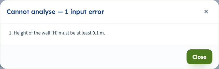
A window titled Cannot analyse — 1 input error (or the number of errors) lists each one, numbered, with the name of the field and its symbol. The bar stays at Not analysed. The messages read:
- “Height of the wall (H) must be at least 0.1 m.” (also for a negative value), or “… is missing.” for an empty box;
- “Thickness (H1) must be at least 0.01 m.”
- “Unit weight above the water table (γ1) must be at least 1 kN/m³.”
- “Drained friction angle (φ′1) must be at most 50°.”, or at least 0° the other way;
- “Overconsolidation ratio (1 = normally consolidated) (OCR1) must be at least 1.”
- “Plasticity index (%) (PI1) must be at least 0.”
- “Coefficient of earth pressure at rest (K0,1) must be at least 0.” or “… must be at most 3.”
- “Depth of the water table below the top (zw) must be at least 0 m.”
The number after a symbol is the layer. Ranges are those of the field tables above. Only the boxes the choices have opened are checked: with Massarsch chosen the friction angle is not asked for.
A condition of the solution
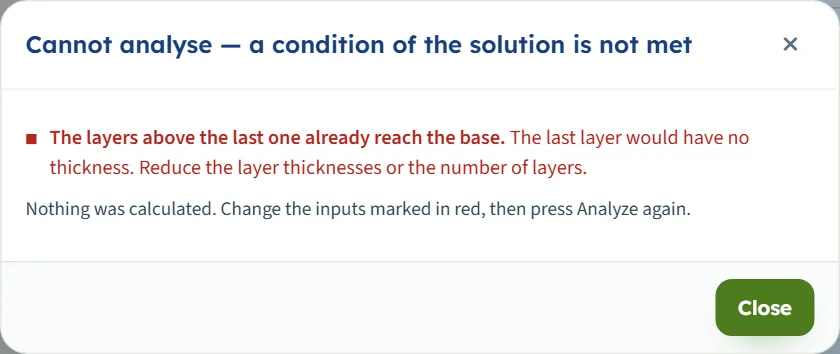
When every value is in range but the model cannot be solved, the window is titled Cannot analyse — a condition of the solution is not met and says “Nothing was calculated. Change the inputs marked in red, then press Analyze again.” The bar turns brown and reads Cannot be analysed followed by the reason. The reasons:
- The layers above the last one already reach the base. “The last layer would have no thickness. Reduce the layer thicknesses or the number of layers.”
- Sherif: the compacted dry unit weight is below the loosest-state value. The window gives both values, for example “Layer 1: the compacted dry unit weight 14.00 kN/m³ is below the loosest-state value 15.00 kN/m³”, and asks for a compacted value not lower than the minimum.
- The saturated unit weight is not above that of water (9.81 kN/m³) in a layer that lies below the water table: the effective unit weight would be zero or negative. Enter the saturated unit weight of the soil. With no water table the saturated weight is not used and this check does not apply.

A caution
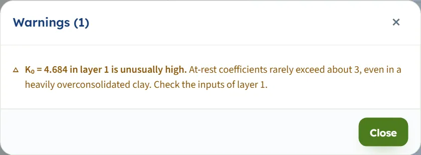
A caution does not stop the run. If K0 of a layer comes out above 3, the analysis runs, the bar reads Analysed — the earth pressure calculated — 1 warning, and a Warnings (1) window opens with the text of the caution. The button Warnings on the bar shows it again; the report prints it. With no cautions the window says “No warnings — the assumptions of the solution hold for these inputs.”
A wall of φ′ = 50° and OCR = 50 gives K0 = 4.684, and a Massarsch layer of OCR = 50 gives 3.705; both trigger it. The module still returns the pressure for that K0. For an entered K0 the limit of the box, 3, applies first.
Good practice and common mistakes
- Use this module for a wall that cannot move. A wall that yields is an active-pressure case, and the pressure is smaller; a wall pushed into the soil is passive. See the other modules of the family.
- Choose K0 by the soil. Jaky for a normally consolidated sand, Mayne–Kulhawy (the same button, with the OCR) for an overconsolidated one, Massarsch for a clay by its PI, Sherif for a compacted fill. Different layers can use different relationships.
- Enter the stress history. A larger OCR raises K0: the example’s OCR of 1.5 gives 0.538 against 0.426 for OCR = 1, and P0 follows.
- Mind the water. Water pushes with its full hydrostatic pressure whatever K0 is, and below the table the soil counts at γsat − γw. Give γsat in every layer that lies below the water table.
- Describe the layers from the top down and let the last one run to the base. A thickness that brings the layers to the base before the last layer stops the module.
- Read P0 per unit length. It is in kN/m; multiply by the length of wall for a total force.
- Add the other actions yourself. A surcharge on the ground behind the wall comes from the Surcharge loads modules; the wall calculation combines it with this pressure.
- Keep a model file. The browser keeps the model as you work, but a file saved with Save to file… is the copy that travels with the project; use Quick Save… to compare variants.
- Check the units after switching the system: type values in the units shown beside the boxes.
Frequently asked questions
What does the at-rest pressure mean?
It is the pressure of the soil on a wall that does not move, so that the soil stays in the state it had in the ground. The horizontal effective stress is K0 times the vertical effective stress. A wall that moves away from the soil gets a smaller pressure (active); one pushed into it gets a larger one (passive).
How is the force on the wall found?
The pressure diagram is built from the stresses at every layer boundary and at the water table, and its area is the force: P0 = Ps + Pw. The height z̄ follows from the moments of the areas about the base. For the module’s example P0 = 92.75 kN/m at 1.422 m.
Which relationship should I choose for K₀?
Jaky / Mayne–Kulhawy for sand and gravel with a measured friction angle, with the OCR for an overconsolidated soil; Massarsch for a clay by its plasticity index; Sherif for a compacted sand fill; Given K₀ for a value of your own, from 0 to 3.
Why is the last layer without a thickness?
The last layer runs on to the base of the wall, so its thickness is the wall height less the layers above. The thickness you type for it is kept and counts as soon as another layer is added below it. If the layers above already reach the base the module stops.
How many layers can I enter?
Up to six, from the top of the wall down. Each has its own unit weights and its own relationship for K0.
How does the water table change the answer?
Below it the soil counts at γsat − γw for the vertical effective stress, and the water adds its hydrostatic pressure u = γw (z − zw). A water table at or below the base gives no water pressure; at the surface the wall is under water over its whole height. Water is taken behind the wall only.
Why did the module stop?
Either a value is outside its range, with a window that names the field, or a condition of the solution is not met: the layers reach the base, a compacted dry unit weight is below the loosest-state value, or a saturated unit weight is not above that of water. Nothing is calculated until you correct it.
What does the caution about K₀ above 3 mean?
It marks a coefficient that is rare even in a heavily overconsolidated clay, so the inputs of that layer deserve a second look. The run is not stopped and the value is used as calculated.
Can I drag the water table or a layer boundary on the drawing?
No. Nothing on the drawing is a handle. Set the wall, the layers and the water table in the Model tab; the drawing follows as you type.
Does the module remember my inputs?
Yes. The model is kept in this browser as you work, so the page opens again where you left it, and an analysed model comes back analysed and locked. For a copy that travels use Save to file…; Quick Save… keeps named versions in the browser; Reset to defaults brings the example back.
Which units does it use?
SI · kN, SI · tf or US, switchable in the header at any time, even after Analyze. The force is in kN/m, tf/m or kip/ft, the pressures in kPa, t/m² or ksf in the tables as the system says, and the heights in m or ft.
Does the result include a surcharge?
No. The result is the pressure of the soil and the water. A load on the ground behind the wall comes from the Surcharge loads modules and is combined with this result in the wall calculation.