

What the module calculates
Coulomb gives the active or passive force of the soil on a retaining wall by Coulomb’s wedge theory (1776). It takes into account the friction between the soil and the wall, a wall back that is not vertical and a backfill that slopes. A plane failure surface runs through the heel of the wall; the module finds the wedge that gives the largest force (active) or the smallest (passive) and reports that force, its two components, the angle of the critical plane and where the force acts.
H is the vertical height of the wall, γ the unit weight, and the coefficient Ka or Kp depends on the friction angle φ′, the wall friction δ′, the inclination θ of the back from the vertical and the slope α of the backfill. The force acts at H/3 above the base for one soil, inclined at δ′ to the normal of the back.
What you can describe
- A wall of vertical height H with its back at θ from the vertical (positive toward the backfill, negative away from it), active (the wall moves away from the soil) or passive (the wall is pushed into it).
- A backfill that rises or falls at α from the horizontal.
- Soil in up to six layers, each with its unit weights, φ′, wall friction δ′ and cohesion c′, with level boundaries.
- A level water table behind the wall, and a uniform surcharge on the backfill surface.
How the modules of the family differ
- One soil, no water, no surcharge: the closed form, its working, and the Trial wedges curve that shows the largest (or smallest) force being picked out.
- Layers, cohesion, a water table or a surcharge: each layer takes its own Coulomb coefficient under the effective vertical stress below the top of the wall, the pressures are summed along the back, and the module reports the force, its inclination, its line of action and, if there is water, the water force. The module states that the layered form is an extension of Coulomb’s solution for one soil.
- The other modules of the family: At rest for a wall that does not move; Rankine and Rankine, sloping backfill for a smooth wall; Mononobe–Okabe for the active force in an earthquake; Passive, log spiral for a curved passive failure surface and Passive, earthquake for passive force in an earthquake.
For a load on the backfill that is not uniform over the whole surface, the Surcharge loads manuals give the pressure it adds to the wall.
Before you start: what you need
Have these ready from your design:
| What | Where it comes from | Notes |
|---|---|---|
| The wall height H | Your design | The vertical height from the top of the wall to its base, at least 0.1 m. |
| The inclination θ of the back | Your design | From −40° to 40°, from the vertical. Positive means the back leans toward the backfill; 0 is a vertical back. |
| The slope α of the backfill | Your design | From −40° to 45°. Positive rises away from the wall. |
| γ, φ′ and c′ of each soil | Tests or correlations | Unit weight above the water table, effective friction angle (above 0°, up to 50°) and effective cohesion (zero for a granular soil). With a water table, also the saturated unit weight. |
| The wall friction δ′ | Your design judgement | The angle of friction between the wall and each layer, from 0° to 45°. The module’s own note: typically φ′/2 to 2φ′/3, and at most φ′. |
| Water table and surcharge | Site data and loading | The depth zw of a level water table below the top of the wall, and a uniform surcharge q on the backfill, if any. |
Quick start in seven steps
- Open the module and choose the units
Open Coulomb from the Lateral Earth Pressure family. Pick SI · kN, SI · tf or US in the header; you can change it at any time.
- Describe the wall
In Wall choose Active or Passive, enter the height H and the inclination θ of the back.
- Describe the backfill
In Backfill enter the slope α.
- Enter the soil
In Soil layers check the first layer (γ, φ′, δ′, c′); to add another, fill in the New layer form and press + Add layer.
- Add water and a surcharge if there are any
In Groundwater choose Present and enter zw; in Surcharge enter q.
- Press Analyze
Press Analyze. The bar reads Analysed — the earth pressure calculated, the inputs lock. Open the Pressure view to see the force.
- Read the answer and take the report
The Results tab gives the force, its components and the critical plane; Calculations writes out the working; Report saves a PDF or a Word file.
The screen: four views of the wall
The layout is the one every GeoTerva module shares, described in the workspace guide: the drawing on the left, the Model, Results, Calculations, Report and Theory tabs on the right, and the unit selector in the header. This module’s drawing has four views, chosen with the buttons above it:
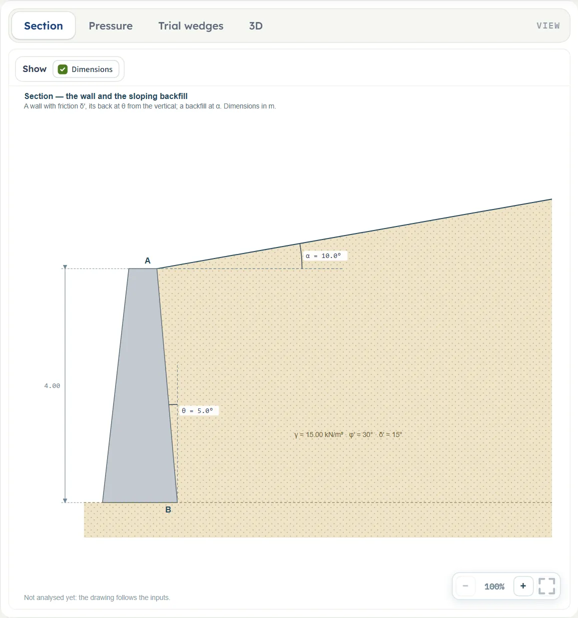
- Section is the geometry alone: the wall, its back at θ, the backfill at α, the layers with their values, the water table and the surcharge. It follows the inputs as you type.
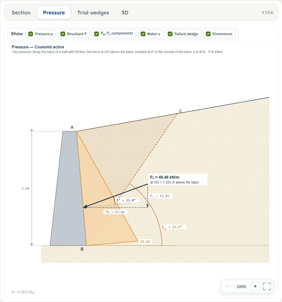
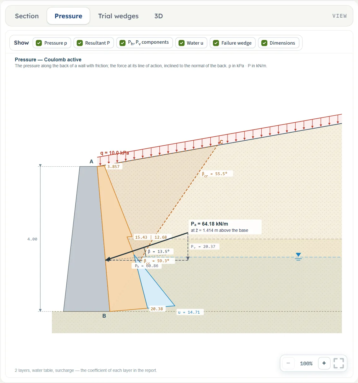
- Pressure shows, after Analyze, the pressure along the back, the water pressure, the resultant force with its components, and the critical failure wedge.
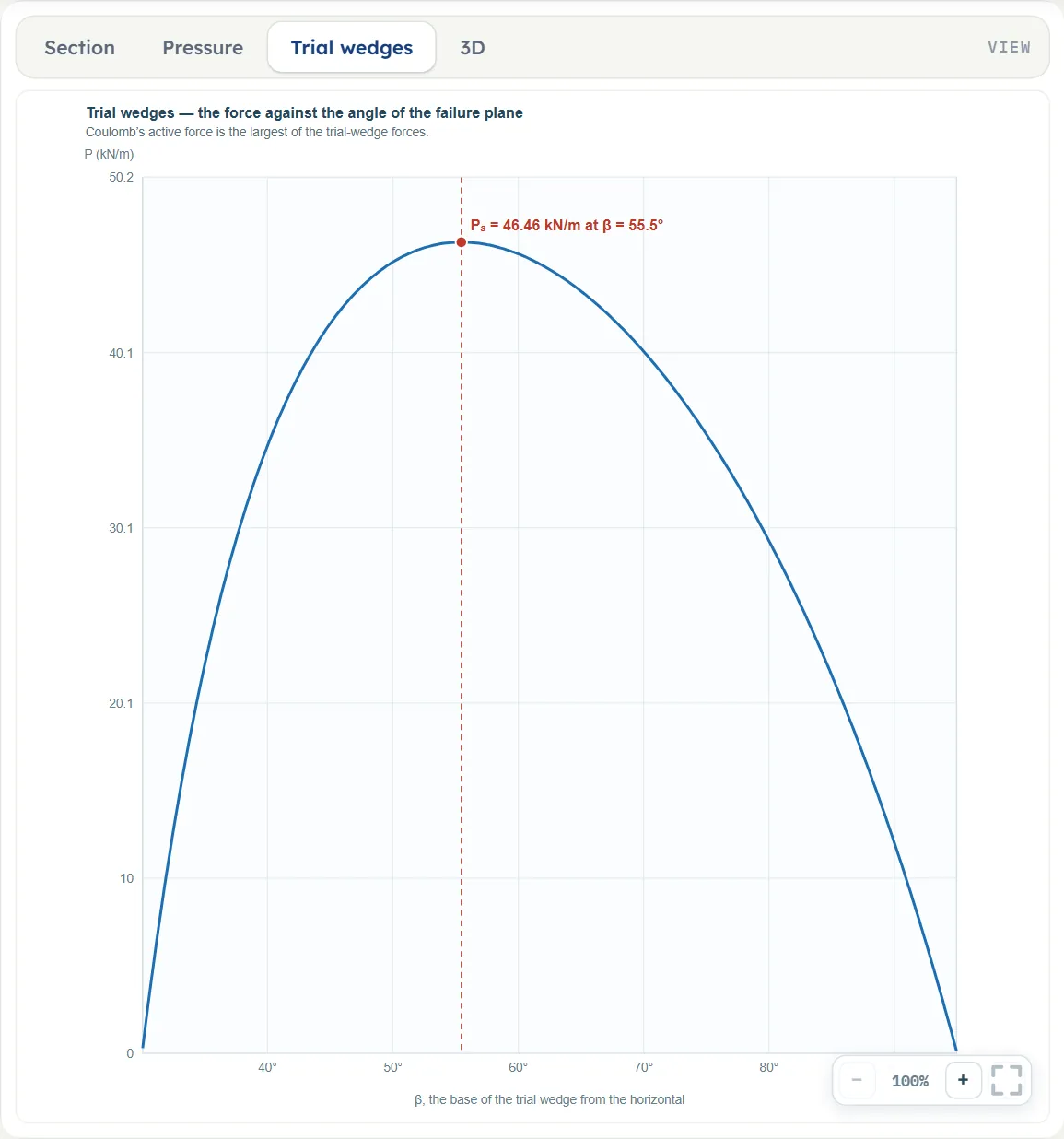
- Trial wedges plots the force of trial wedges against the angle β of their base plane, with the critical wedge marked. It is drawn for one soil without water or a surcharge.
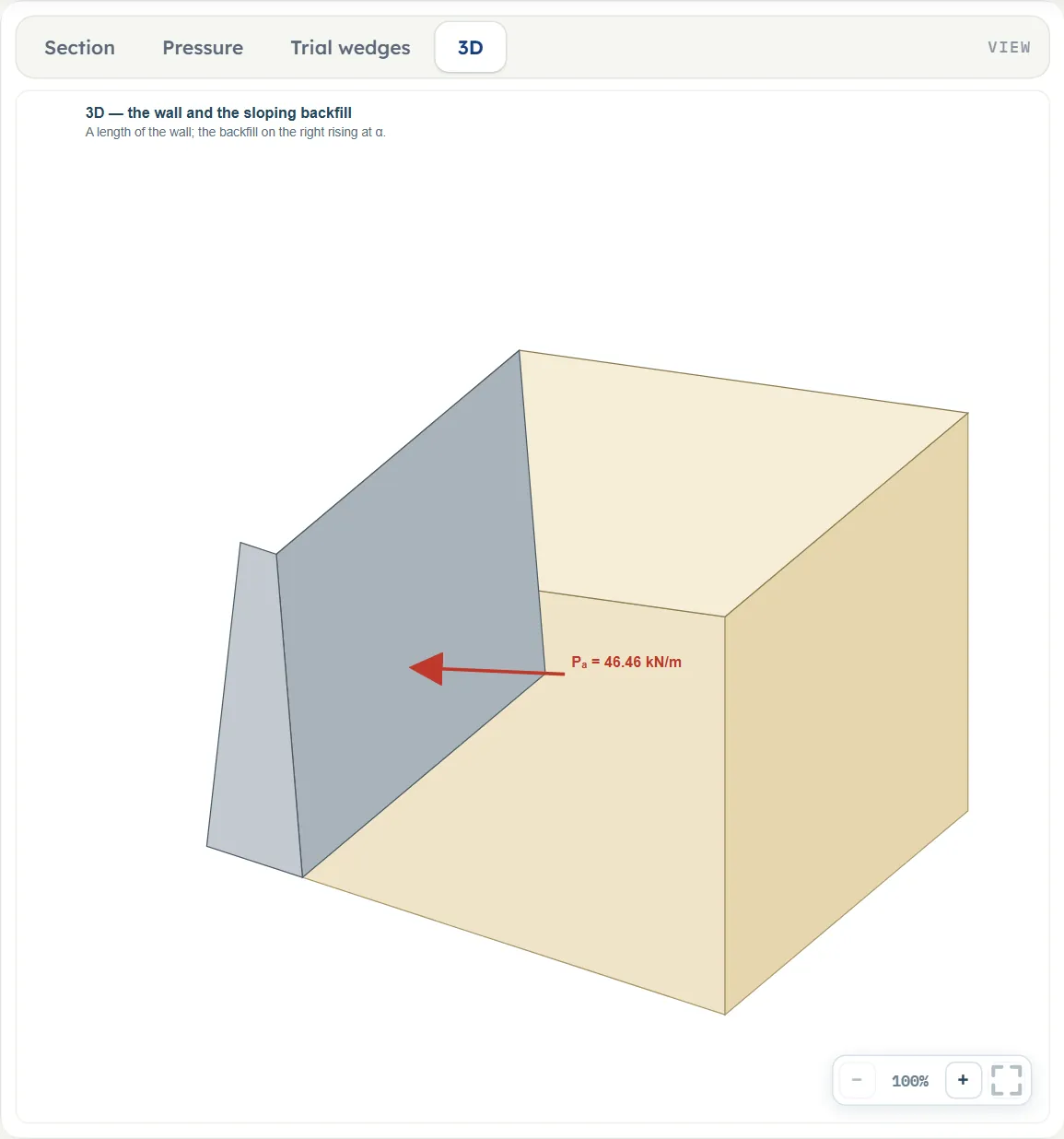
- 3D shows a length of the wall with the sloping backfill, and the force after Analyze.
The Show chips
A Show bar above the drawing switches elements on and off. In Section there is one chip, Dimensions. In Pressure there are six: Pressure p, Resultant P, Ph, Pv components, Water u, Failure wedge and Dimensions. Before Analyze the Pressure view shows the geometry only and says “The pressures and the resultant appear after Analyze”.
Zoom, and nothing to change by dragging
Each view has − and + zoom buttons with the zoom shown between them, and a button that fits the whole drawing in the pane. Nothing on the drawing can be dragged to change a value: every number is entered in the Model tab, and the drawing follows. When zoomed in, drag the drawing to move it. After Analyze the inputs are locked.
Entering the model, section by section
The Model tab starts with Model data (the same in every module; see the workspace guide) and then has five sections: Wall, Backfill, Soil layers, Groundwater and Surcharge. Each opens when you click its title; Next and Back walk you through them. Where a unit is shown twice or three times, such as m · ft, the units are those of SI · kN, SI · tf and US in turn, and equal ones are merged. Defaults are shown in SI; after you switch units the boxes convert the same wall and soil, for example γ = 1.52957 t/m³ in SI · tf and H = 13.1234 ft, γ = 95.4882 pcf in US.
Wall
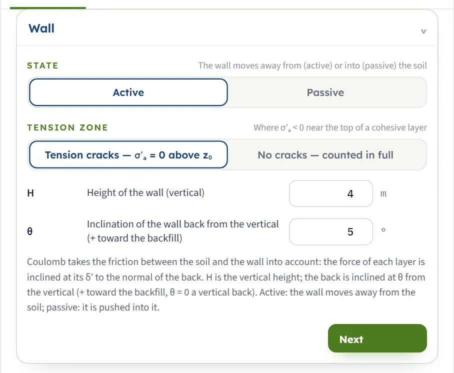
Two choices and two numbers. State is Active (the wall moves away from the soil, the default) or Passive (the wall is pushed into it). Tension zone appears for the active state and is explained under soil with cohesion.
| Field | Unit | Default | What to enter |
|---|---|---|---|
| Height of the wall (vertical) H | m · ft | 4 | The vertical height of the wall. At least 0.1 m; a blank box stops the analysis. |
| Inclination of the wall back from the vertical (+ toward the backfill) θ | ° | 5 | From −40° to 40°. 0 is a vertical back. |
Backfill
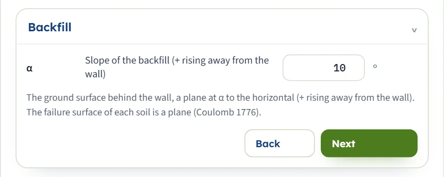
One number: the slope of the ground surface behind the wall. A plane surface at α to the horizontal, positive when it rises away from the wall.
| Field | Unit | Default | What to enter |
|---|---|---|---|
| Slope of the backfill (+ rising away from the wall) α | ° | 10 | From −40° to 45°. |
Soil layers
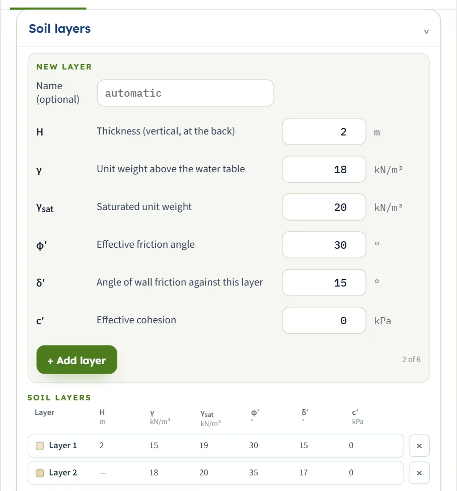
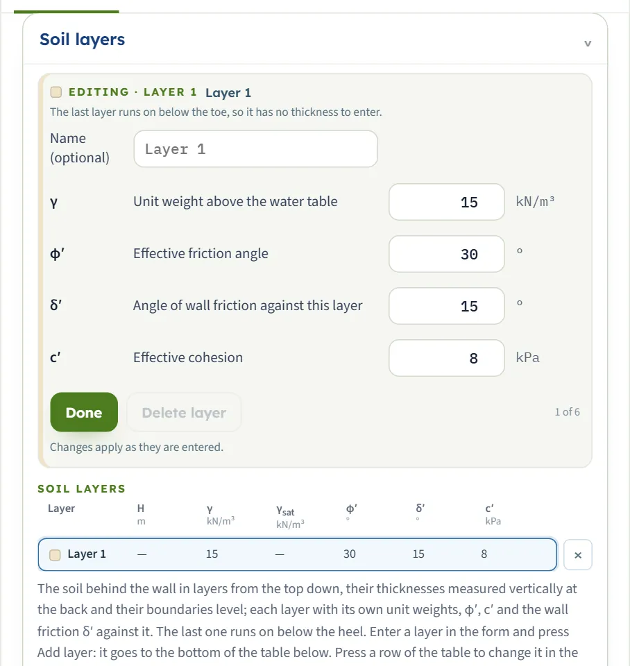
The soil behind the wall goes in from the top down. The module opens with one layer. To add another, fill in the New layer form and press + Add layer: it goes to the bottom of the Soil layers table below, and the counter (“2 of 6”) moves on. Up to six layers can be entered.
The Default column is the first layer, which the module opens with. The New layer form opens with γ = 18 kN/m³, γsat = 20 kN/m³, φ′ = 30°, δ′ = 15°, c′ = 0 and thickness 2 m.
| Field | Unit | Default | What to enter |
|---|---|---|---|
| Name | — | empty | Labelled Name (optional); the box shows “automatic” when empty. Shown on the drawing and in the tables; leave blank for the automatic name (Layer 1, Layer 2, …). |
| Thickness (vertical, at the back) Hi | m · ft | 2 | Measured vertically at the back of the wall from its top; the boundaries are level. At least 0.01 m. The last layer has no thickness: it runs on below the heel. Shown when there is more than one layer. |
| Unit weight above the water table γ | kN/m³ · t/m³ · pcf | 15 | At least 1 kN/m³. |
| Saturated unit weight γsat | kN/m³ · t/m³ · pcf | 19 | Used below the water table, where the layer weighs γ′ = γsat − γw. Must be above that of water (9.81 kN/m³). Shown when the water table is present. |
| Effective friction angle φ′ | ° | 30 | Above 0°, up to 50°. |
| Angle of wall friction against this layer δ′ | ° | 15 | From 0° to 45°. Typically φ′/2 to 2φ′/3, at most φ′. |
| Effective cohesion c′ | kPa · kg/cm² · psf | 0 | Zero for a granular soil. A value above zero adds the cohesion term to the pressure of that layer. |
To change a layer, press its row in the table. The form opens with Editing · Layer n in its title; changes apply as you type, Done closes it and Delete layer removes it. The × at the end of a row removes a layer too (not the last one left). The last layer has no thickness to enter: it runs on below the heel of the wall. The layers above it must not already reach the base.
Groundwater
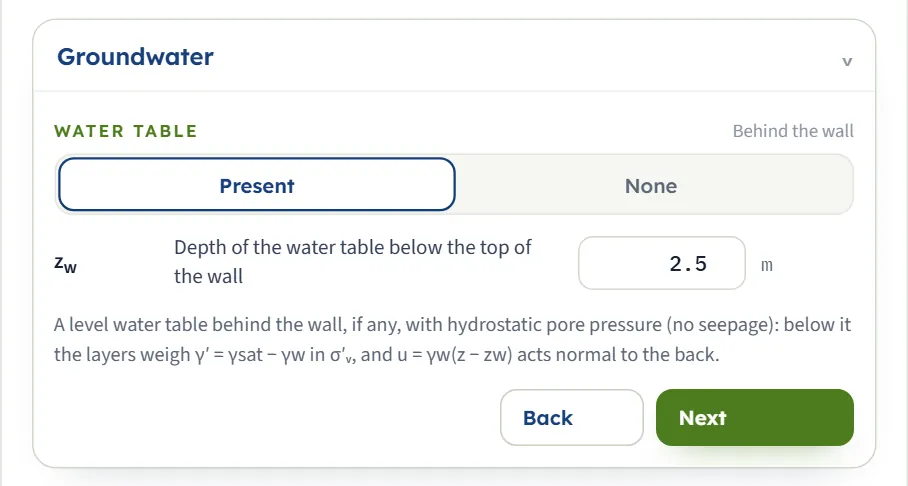
Water table is None (the default) or Present. With water present the depth zw is asked for, and each layer asks for its saturated unit weight. The table is level, the pore pressure hydrostatic (no seepage): below the water table the layers weigh γ′ = γsat − γw in the effective vertical stress, and the pore pressure u acts normal to the back.
| Field | Unit | Default | What to enter |
|---|---|---|---|
| Depth of the water table below the top of the wall zw | m · ft | 2 | At least 0. A table at or below the base of the wall has no effect. Shown when Water table is Present. |
Surcharge
A uniform surcharge on the backfill surface. In the wedge it acts as the vertical stress q cos θ / cos(θ − α) added at every depth.

| Field | Unit | Default | What to enter |
|---|---|---|---|
| Uniform surcharge on the backfill surface q | kPa · t/m² · ksf | 0 | Vertical, per unit area of the sloping surface. Zero or more; 0 for none. |
Choosing the state, the angles and the soil model
Active or passive. Choose Active when the wall moves away from the soil, so that the soil pushes it; choose Passive when the wall is pushed into the soil and the soil resists. The example gives Ka = 0.3872 and Pa = 46.46 kN/m active, and Kp = 6.732 and Pp = 807.9 kN/m passive, for the same wall and soil.
The wall friction δ′. It turns the force away from the normal of the back, and it changes the coefficient. The module’s note is that δ′ is typically φ′/2 to 2φ′/3 and never more than φ′. For the active case the coefficient changes little in that range; for the passive case it grows quickly with δ′: the example gives Kp = 5.393 with δ′ = 10° and 6.732 with 15°. With δ′ above φ′/2 in the passive state, the module cautions that the real failure surface is curved and the plane of Coulomb overestimates the force, and points to the Passive, log spiral module.
The back and the slope. A back leaning toward the backfill (θ positive) and a backfill that rises (α positive) both increase the active force; the “How each input changes the answer” table shows by how much. The active case has a solution only for α ≤ φ′, and a back no steeper than φ′ has no active wedge.
One soil, or layers, water and a surcharge
The module chooses the way of working by what you enter:
| Model | What you get | Results tab |
|---|---|---|
| One layer, no cohesion, no water, no surcharge | Coulomb’s closed form: K, P = ½ γ H² K, at H/3, inclined at δ′; the Trial wedges curve | Force, K, the two components, βcr |
| Layers, cohesion, a water table or a surcharge | Each layer takes its own K under the effective vertical stress; the pressures are summed along the back | Force, inclination β to the normal, line of action z̄, components, the water force Pw and the depth z0 of a tension zone where they apply |
The same wall as a one-layer model and as a layered one agree: a single layer with nothing else switched on reduces to the closed form.
Soil with cohesion and the tension zone
A layer with c′ above zero takes the pressure σ′ = K σ′v − 2c′√K (active) or K σ′v + 2c′√K (passive), with the Coulomb coefficient of the layer; the module neglects the adhesion between wall and soil. In the active state the pressure is negative near the top of a cohesive layer. Tension zone decides what happens there:
- Tension cracks — σ′ₐ = 0 above z₀ (the default): the soil cannot pull on the wall, so no pressure acts above z0, the depth where the pressure first becomes positive.
- No cracks — counted in full: the soil is taken to stay in contact with the wall, and the negative area is subtracted from the force.
Example (a 4 m vertical wall, level backfill, φ′ = 26°, c′ = 8 kPa, γ = 15 kN/m³, δ′ = 0): Ka = tan²(32°) = 0.3905, z0 = 2c′/(γ√Ka) = 16/(15 × 0.6249) = 1.707 m, which is the depth the module gives (1.707 m), and the force with cracks is 15.40 kN/m.
Analyze and read the results
Press Analyze. The bar at the foot of the Model tab changes to Analysed — the earth pressure calculated and says “The inputs are locked. Edit inputs clears the results; the unit system can still be changed.” Edit inputs unlocks the model and clears the results; Warnings (with the number of them) lists the cautions of the run, and a window with them opens when there are any.
One soil: the cards
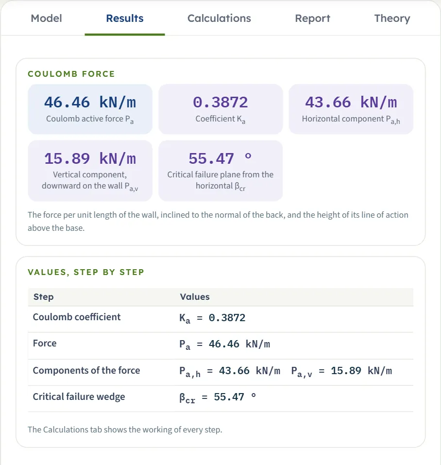
| Card | Symbol | The example |
|---|---|---|
| Coulomb active force (or passive) | Pa (Pp) | 46.46 kN/m |
| Coefficient | Ka (Kp) | 0.3872 |
| Horizontal component | Pa,h | 43.66 kN/m |
| Vertical component, downward (active) or upward (passive) on the wall | Pa,v | 15.89 kN/m |
| Critical failure plane from the horizontal | βcr | 55.47 ° |
The force is per unit length of the wall. The components are Ph = P cos(δ′ + θ) and Pv = P sin(δ′ + θ) in the active state (with δ′ − θ in the passive state): 46.46 × cos 20° = 43.66 kN/m and 46.46 × sin 20° = 15.89 kN/m.
Layers, water or a surcharge: the cards and the tables
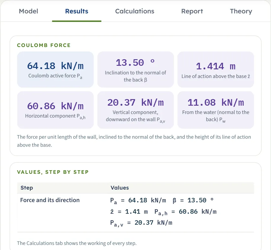
The cards become the force P, its inclination β to the normal of the back, the line of action z̄ above the base, the two components, the water force Pw (normal to the back) when there is water, and the depth z0 of the tension zone when a cohesive layer has one. Below them are tables: The layers and their Coulomb coefficient (with K and βcr of each layer), Stresses on the back, and Force of each layer (the normal and tangential parts of each).
The Trial wedges view
For one soil without water or a surcharge, Trial wedges plots the force of the wedge whose base plane is at β. The active force is the largest of the trial-wedge forces and the passive force the smallest; the critical wedge is marked, here Pa = 46.46 kN/m at β = 55.5°. When layers, water or a surcharge are present the view says that the trial wedges are drawn for one soil without them, and that the report lists the coefficient of each layer.
The Calculations tab, the report and the Theory tab
The Calculations tab writes out the working. It starts with Given and what is sought, then follows the steps:
- One soil (four steps): the Coulomb coefficient with its numbers; the force P = ½ γ H² K at H/3, inclined at δ′; the components of the force; and the critical failure wedge with βcr . A closing Answer gives K and P.
- Layers, cohesion, water or a surcharge: the Coulomb coefficient of each layer with a table of the layers; the stresses on the back (with a table of σ′v, σ′ and u); the tension zone when a cohesive layer has one, with the force the other assumption would give; the force and its direction, with the force of each layer; and the critical failure plane of each layer.
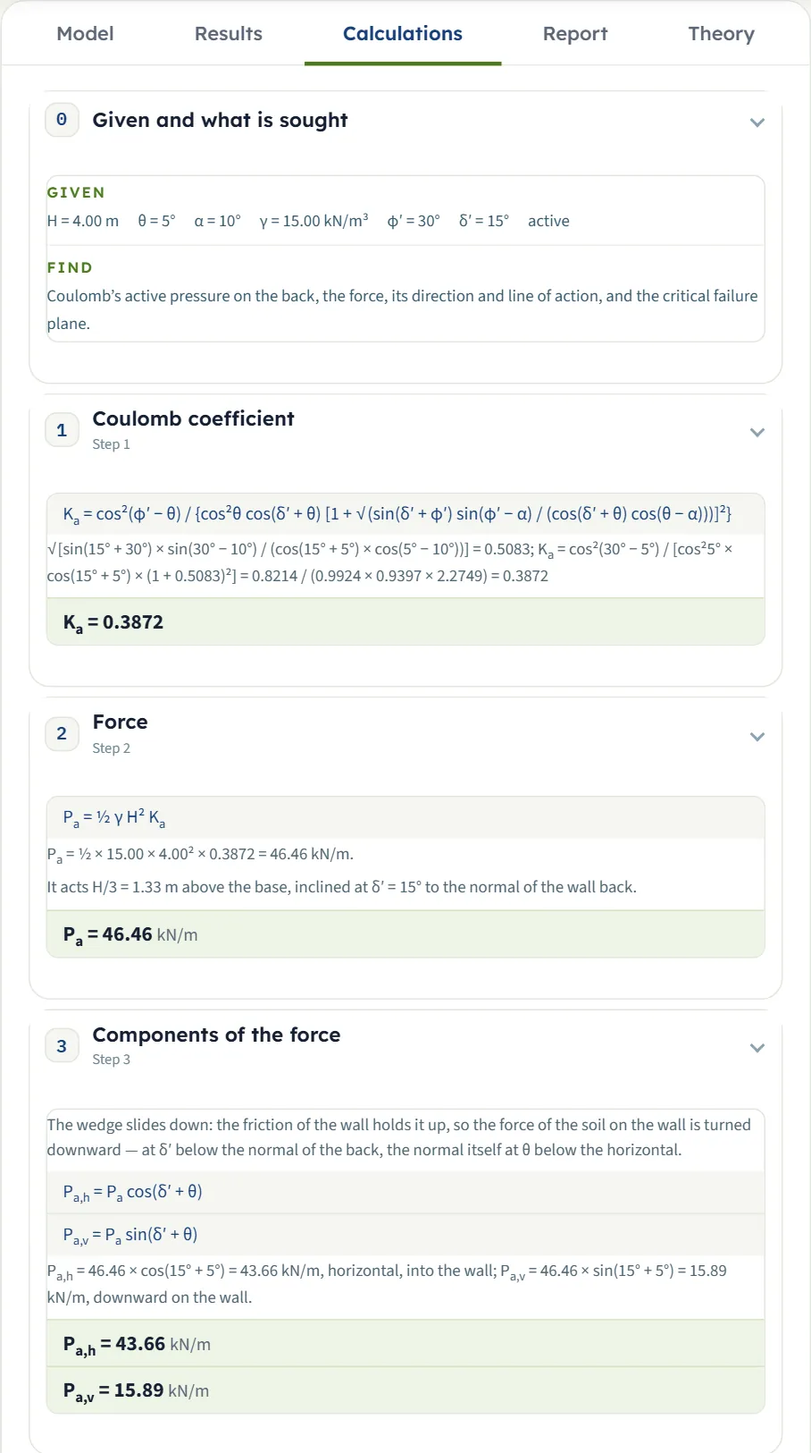
Every number on the Results tab can be traced to a step here.
The report
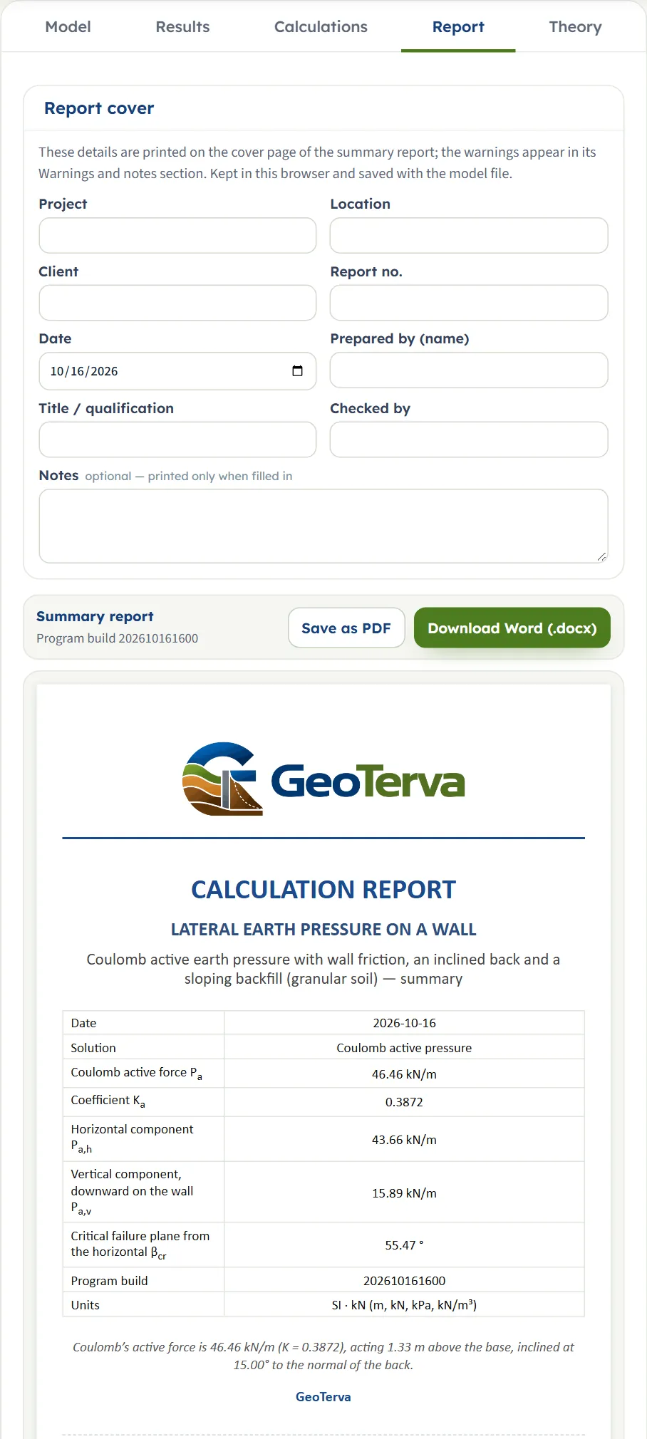
In the Report tab fill in the cover (project, location, client, report number, date, prepared by, title / qualification, checked by, and optional notes). After Analyze Save as PDF and Download Word (.docx) work; the preview below the buttons is the report itself.
The report has six parts: 1 Introduction and scope, 2 Input data, 3 Calculation (for one soil: 3.1 Coulomb coefficient, 3.2 Force, 3.3 Components of the force, 3.4 Critical failure wedge), 4 Results, 5 Summary and 6 References. It carries the drawings, states the units with their conversion constants and prints the warnings of the run.
The Theory tab
The Theory tab has six sections: The trial wedge, Coulomb’s active pressure, Coulomb’s passive pressure, Layers, water and surcharge, a worked example, and References.
Worked example: the module’s own example
The module opens on this example (after Reset to defaults), so you can follow the numbers on your own screen.
| Section | Input | Value |
|---|---|---|
| Wall | State, height, back | Active; H = 4 m; θ = 5° |
| Backfill | Slope | α = 10° |
| Soil layers | One layer | γ = 15 kN/m³; φ′ = 30°; δ′ = 15°; c′ = 0 |
| Groundwater, Surcharge | None | Water table None; q = 0 |
Step 1: the coefficient
The square root term is √[sin(15° + 30°) sin(30° − 10°) / (cos(15° + 5°) cos(5° − 10°))] = 0.5083, so
Step 2: the force
It acts H/3 = 1.33 m above the base, inclined at δ′ = 15° to the normal of the back.
Step 3: the components
Pa,h = 46.46 × cos(15° + 5°) = 43.66 kN/m (horizontal, into the wall); Pa,v = 46.46 × sin 20° = 15.89 kN/m (downward on the wall).
Step 4: the critical plane
The critical wedge has βcr = 55.47° to the horizontal, and its force is the same 46.46 kN/m as from Ka.
The same wall, passive
Choose Passive: Kp = 6.732, Pp = ½ × 15 × 16 × 6.732 = 807.9 kN/m, with Pp,h = 795.6 kN/m and Pp,v = 140.3 kN/m upward on the wall and βcr = 29.56°. Here δ′ = 15° equals φ′/2, so there is no caution; a δ′ of 20° brings one (see Messages).
A check with a vertical back and a level backfill
With θ = 0, α = 0, δ′ = 20°, H = 5 m, γ = 18 kN/m³ and φ′ = 30° the module gives Ka = 0.2973 and Pa = 66.90 kN/m, which is ½ × 18 × 25 × 0.2973 by hand. Passive, with δ′ = 15°: Kp = 4.977 and Pp = 1,120 kN/m (½ × 18 × 25 × 4.977 = 1,120).
The same wall in other units
In SI · tf the module gives Pa = 4.738 tf/m (46.46 kN/m ÷ 9.80665). In US, switching converts the boxes to H = 13.1234 ft and γ = 95.4882 pcf, and the module gives Pa = 3.184 kip/ft, Pa,h = 2.992 kip/ft and Pa,v = 1.089 kip/ft, with Ka = 0.3872 and βcr = 55.47° unchanged. Typing the rounded 13.12 ft and 95.49 pcf instead gives 3.182 kip/ft.
With a surcharge
Enter q = 10 kPa. The module now works in its layered form and gives Pa = 61.95 kN/m inclined at 15.00° (that is δ′) with the line of action z̄ = 1.500 m. By hand: the stress added is q cos 5° / cos(5° − 10°) = 10 kPa, so Pa = Ka (q H + ½ γ H²) = 0.3872 × (40 + 120) = 61.95 kN/m, and the moments about the base give (15.49 × 2 + 46.46 × 1.333) / 61.95 = 1.50 m.
How each input changes the answer
Each row changes one thing in the example and runs the module again; the numbers are the ones the module gives, so you can reproduce any row. First, one soil without water or a surcharge:
| Change | K | P | Ph | Pv |
|---|---|---|---|---|
| The example: active, φ′ = 30°, δ′ = 15°, θ = 5°, α = 10° | 0.3872 | 46.46 | 43.66 | 15.89 |
| δ′ = 0 | 0.4149 | 49.79 | 49.60 | 4.339 |
| δ′ = 20° | 0.3857 | 46.29 | 41.95 | 19.56 |
| δ′ = 30° | 0.3935 | 47.22 | 38.68 | 27.08 |
| φ′ = 25° | 0.4686 | 56.23 | 52.84 | 19.23 |
| φ′ = 35° | 0.3189 | 38.27 | 35.96 | 13.09 |
| φ′ = 40° | 0.2607 | 31.28 | 29.39 | 10.70 |
| α = 0° | 0.3379 | 40.55 | 38.10 | 13.87 |
| α = 20° | 0.4708 | 56.50 | 53.09 | 19.32 |
| α = 30° (= φ′) | 0.8808 | 105.7 | 99.32 | 36.15 |
| θ = 0° | 0.3432 | 41.18 | 39.78 | 10.66 |
| θ = 15° | 0.4936 | 59.23 | 51.30 | 29.62 |
| θ = −10° | 0.2670 | 32.04 | 31.92 | 2.792 |
| H = 6 m | 0.3872 | 104.5 | 98.23 | 35.75 |
| γ = 18 kN/m³ | 0.3872 | 55.75 | 52.39 | 19.07 |
| Passive state | 6.732 | 807.9 | 795.6 | 140.3 |
- φ′: a larger friction angle gives a smaller coefficient and force: Ka falls from 0.4686 at 25° to 0.2607 at 40°.
- δ′: the active force changes little with wall friction (49.79, 46.46 and 47.22 kN/m for 0°, 15° and 30°), but the vertical component grows from 4.339 to 27.08 kN/m.
- α and θ: a rising backfill and a back leaning toward the fill raise the active force. At α = φ′ the force is 105.7 kN/m, with the critical plane parallel to the surface (βcr = 30.00°).
- H and γ: the force is proportional to γ and to H²: 46.46 × (6/4)² = 104.5 kN/m, and 46.46 × 18/15 = 55.75 kN/m.
Now water and a surcharge (the module works in its layered form, so the cards are the force, its inclination β to the normal, the line of action z̄ and the water force):
| Change | P (kN/m) | β (°) | z̄ (m) | Pw (kN/m) |
|---|---|---|---|---|
| q = 10 kPa | 61.95 | 15.00 | 1.500 | — |
| Two layers (lower: 18 kN/m³, 35°, 17°) and q = 10 kPa | 56.26 | 16.31 | 1.556 | — |
| The same with a water table at 2.5 m | 64.18 | 13.50 | 1.414 | 11.08 |
| Water table at zw = 1 m (one soil) | 79.97 | 6.754 | 1.188 | 44.31 |
| Water table at zw = 2 m (one soil) | 61.20 | 10.22 | 1.163 | 19.69 |
| Water table at zw = 3 m (one soil) | 50.11 | 13.54 | 1.255 | 4.924 |
- A surcharge adds K qe H to the force, where qe = q cos θ / cos(θ − α) (equal to q in this example), and moves its line of action up (from 1.333 m to 1.500 m).
- Water adds its own force normal to the back and lowers the effective weight of the soil below it: the shallower the table, the larger the total force (79.97, 61.20 and 50.11 kN/m for 1, 2 and 3 m, against 46.46 without water).
Messages: when the module stops, and cautions
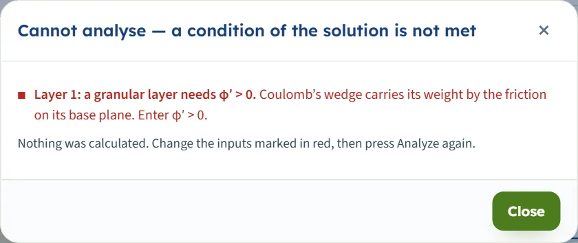
When a value cannot be used the module stops and nothing is calculated. A window titled Cannot analyse lists what is wrong; it says either “1 input error” (a value missing or outside its range) or “a condition of the solution is not met” (angles or layers that admit no solution), and the second kind ends with “Nothing was calculated. Change the inputs marked in red, then press Analyze again.”
The input errors name the field and the limit:
- “Height of the wall (vertical) (H) must be at least 0.1 m.” (and “… is missing.” for an empty box).
- “Slope of the backfill … (α) must be at most 45°.” and, in the same form, the limit of θ (40°), and “Uniform surcharge … (q) must be at least 0 kPa.”
| Kind | When | What to do |
|---|---|---|
| Stop | φ′ is 0: “Layer 1: a granular layer needs φ′ > 0.” | Enter φ′ above 0; Coulomb’s wedge carries its weight by friction on its base plane. |
| Stop | Active, α above φ′: “no Coulomb solution for these angles … the backfill is steeper than φ′ (α > φ′).” | Reduce α to φ′ or less. |
| Stop | Active, the back no steeper than φ′: “no active wedge — the back is no steeper than φ′.” | Increase θ or reduce φ′. |
| Stop | Passive, α below −φ′: “no Coulomb solution for these angles”; or φ′ + δ′ + α − θ reaches 90° | Use α ≥ −φ′; reduce δ′ or α, or increase θ. |
| Stop | The layers above the last one reach the base: “The layers above the last one already reach the base.” | Reduce the thicknesses or the number of layers. |
| Stop | With water, a saturated unit weight not above 9.81 kN/m³: “the saturated unit weight … is not above that of water.” | Enter the saturated unit weight of the soil. |
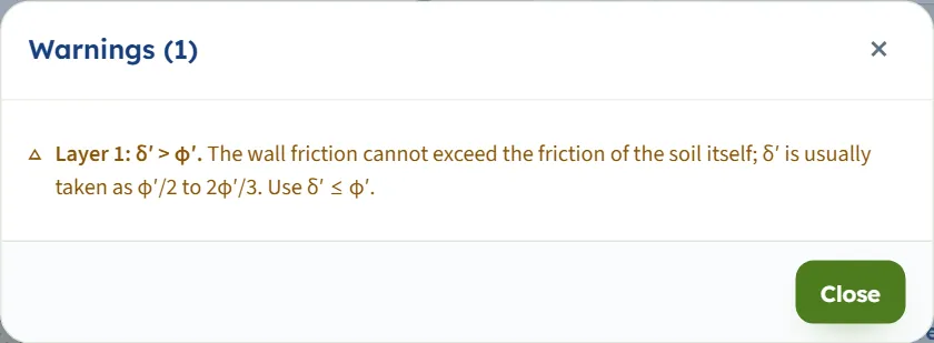
| Caution | δ′ above φ′: “Layer 1: δ′ > φ′.” | The wall friction cannot exceed that of the soil; use δ′ ≤ φ′. |
| Caution | Passive, δ′ above φ′/2: “Coulomb’s passive force with δ′ > φ′/2.” | The real failure surface is curved and the plane overestimates the force; consider the log-spiral module. |
| Caution | Active, cohesive layer, “No cracks” chosen, and the tension outweighs the pressure: “The net active force has no line of action on the wall.” | Tension cracks give the pressure on a wall the soil cannot pull. |
A caution does not stop the analysis: the results appear and a Warnings window opens with the text; the same text is printed in the report.
Good practice and common mistakes
- Choose δ′ deliberately. Use the typical φ′/2 to 2φ′/3. In the passive state it matters most: the force grows quickly with δ′ (Kp from 5.393 at 10° to 6.732 at 15° in the example), and above φ′/2 the plane of Coulomb overestimates it.
- Measure the wall from its top. H is the vertical height; the layers’ thicknesses are measured vertically at the back, from the top of the wall, with level boundaries.
- Mind the sign of θ and α. θ is positive when the back leans toward the backfill, α is positive when the ground rises away from the wall.
- Remember the force is inclined. It acts at δ′ to the normal of the back; use the horizontal and vertical components Ph and Pv in the stability checks, and the line of action given.
- Check the saturated unit weight when you add water: it must be above 9.81 kN/m³, and it is asked for in every layer.
- Do not enter a load that does not cover the surface as q. q covers the whole backfill surface; for a strip, a line or a point load use the Surcharge loads modules and add their pressure to this force.
- Run active and passive separately. They are different states of the wall; the module analyses one at a time.
- Read the Warnings. A caution tells you where the model leaves the range where Coulomb’s plane is reliable.
Frequently asked questions
How is Coulomb’s active force calculated?
A plane failure surface runs through the heel; the force on the wall follows from the equilibrium of the wedge (its weight, the reaction on the failure plane at φ′ to its normal, and the wall force at δ′ to the normal of the back). The critical wedge gives the largest force: Pa = ½ γ H² Ka. For the module’s example, Ka = 0.3872 and Pa = 46.46 kN/m at H/3, inclined at 15° to the normal of the back.
What is the difference between Coulomb and Rankine?
Rankine assumes a smooth wall and a force parallel to the backfill. Coulomb takes the friction δ′ between the soil and the wall into account, and the inclination θ of the back. With δ′ = 0, θ = 0 and a level backfill the two coefficients are the same.
What do θ and α mean, and which sign is which?
θ is the inclination of the back from the vertical, positive when it leans toward the backfill; α is the slope of the backfill from the horizontal, positive when it rises away from the wall. θ is limited to ±40°, α from −40° to 45°.
What value of the wall friction should I enter?
The module’s note: typically φ′/2 to 2φ′/3 and at most φ′. A δ′ above φ′ is accepted with a caution. For the passive state, a δ′ above φ′/2 brings a caution that Coulomb’s plane overestimates the force.
Can I use layers, water and a surcharge?
Yes: up to six layers with level boundaries, a level water table and a uniform surcharge on the backfill. Each layer takes its own Coulomb coefficient under the effective vertical stress below the top of the wall, and the pressures are summed along the back. The module states that this layered form is an extension of Coulomb’s solution for one soil.
Does the module handle cohesion?
Yes: a layer with c′ above zero takes the pressure K σ′v − 2c′√K (active) or + 2c′√K (passive), neglecting the adhesion between wall and soil. In the active state the Tension zone choice decides whether the soil above z₀ is taken to lose contact with the wall (the default) or to stay in contact.
Where does the force act, and in what direction?
For one soil it acts H/3 above the base, inclined at δ′ to the normal of the back. With layers, cohesion, water or a surcharge the module gives the line of action z̄ above the base and the inclination β to the normal. The Results tab gives the horizontal and vertical components, and says whether the vertical one is downward (active) or upward (passive) on the wall.
Why does the Trial wedges view show no curve?
The curve is drawn for one soil without water or a surcharge. With layers, a water table or a surcharge the view says so, and the coefficient of each layer is listed on the Results tab and in the report.
What values stop the analysis?
A wall height under 0.1 m or empty, φ′ of 0, a backfill steeper than φ′ in the active state, a back no steeper than φ′, a passive case whose angles leave no wedge, layers that reach the base, or a saturated unit weight not above that of water. The window names the value and what to change.
Can I drag the wall or the backfill on the drawing?
No. Nothing on the drawing can be dragged to change a value; when zoomed in, drag the drawing to move it. Enter every number in the Model tab and the drawing follows. After Analyze the inputs are locked until you press Edit inputs.
Does the module remember my inputs?
Yes. The model, its analysed state and the unit system are kept in the browser, so the page opens again on the model you last worked on; Reset to defaults brings the example back. For a copy that travels use Save to file…, and Quick Save… for named versions in the browser.
Which units does it use, and what does it give?
SI · kN, SI · tf or US, switchable at any time, even after Analyze. The force per unit length is in kN/m, tf/m or kip/ft, the pressures in kPa, t/m² or ksf, the angles in degrees. For the example 46.46 kN/m is 4.738 tf/m, and in US units (the boxes convert to 13.1234 ft and 95.4882 pcf) 3.184 kip/ft; typing the rounded 13.12 ft and 95.49 pcf gives 3.182 kip/ft.