

What the module calculates
Strip load gives the extra lateral pressure on a wall from a uniform load on a long strip of the ground behind it. You give the height of the wall, the distance of the near and the far edge of the strip from the wall and the load per unit area; the module gives the pressure at every depth, its resultant PH per unit length of wall, the depth zR at which the resultant acts, and the peak pressure with its depth.
The strip is long and parallel to the wall, so the problem is two-dimensional and every result is per unit length of wall. At a depth z the two rays from the point of the wall to the edges of the strip make the angles that give the pressure:
β is the angle the strip subtends at the wall point, α is the angle of its bisector from the vertical and ψ depends on the method you choose: 2 for a rigid wall, 1 for the half-space (a wall that gives way). The resultant is the area of the pressure diagram over the height of the wall, and zR is the depth below the ground at which the first moment of the diagram balances.
What you can describe
- A wall of any height H, with the ground surface level with its top.
- A strip from x1 to x2 measured from the wall, with a uniform load q. The strip may start at the wall face (x1 = 0).
- Two methods: Elastic · rigid wall (the default) and Elastic · half-space.
- SI · kN, SI · tf or US units, switchable at any time.
What you get
- The pressure diagram on the wall, drawn in elevation, in plan and in 3D, with the resultant and its level.
- The resultant force PH per unit length of wall and its depth zR, the peak pressure σH,max and the depth of the peak.
- The working step by step, with a table of the pressure at 31 depths, and a summary report as PDF or Word.
What belongs to other modules
- Other shapes of load have a module each: a point load, a line load, a triangular load, a uniform surcharge, rectangular areas and a ramp load.
- This module gives the pressure that the strip adds. No soil properties are asked: the elastic strip-load solution depends on the geometry and the load only.
- The load is a surface load on a long strip. The result is the horizontal pressure and its resultant on the wall: the surcharge component, to be combined with the earth, water and other actions of your wall analysis.
Before you start: what you need
Four numbers and one decision are enough:
| What | Where it comes from | Notes |
|---|---|---|
| Wall height H | Your design | The height over which the pressure is added up, measured from the ground surface down. It must be greater than zero. |
| Near edge x1 | The layout of the load | The distance from the wall to the edge of the strip nearer to it. Zero or more; zero puts the edge at the wall face. |
| Far edge x2 | The layout of the load | The distance from the wall to the farther edge. It must lie beyond x1; the width of the strip is b = x2 − x1. |
| Strip load q | Your design basis | The load per unit area on the strip, zero or more. |
| The method | How the wall behaves | Elastic · rigid wall is for a wall that does not yield; Elastic · half-space for a wall that deflects enough to relieve the soil. |
Quick start in eight steps
- Open the module and choose the units
Open Strip load from the Surcharge Loads family. Pick SI · kN, SI · tf or US in the header; you can change it at any time. Open Strip load.
- Enter the wall height
In Geometry, type the wall height H.
- Place the strip
In Geometry, type the near edge x1 and the far edge x2, or drag the edges or the body of the strip on the drawing.
- Enter the load
In Strip load, type the load q on the strip.
- Choose the method
In Method, pick Elastic · rigid wall or Elastic · half-space. The (?) beside each opens a drawing of the pressure and the formula.
- Press Analyze
Press Analyze. The bar turns green and reads Analysed, the inputs lock, and the pressure diagram and the resultant appear on the drawing.
- Read the answer
The Results tab gives the strip width, the method, the resultant PH and its depth zR, the peak pressure and its depth. Switch the drawing between Elevation, Plan and 3D View.
- Check the working and take the report
The Calculations tab shows every step; the Report tab saves a PDF or a Word file.
The screen: three views, the Show chips and dragging
The layout is the one every GeoTerva module shares, described in the workspace guide. For this module the drawing on the left has three views, chosen with the buttons above it:
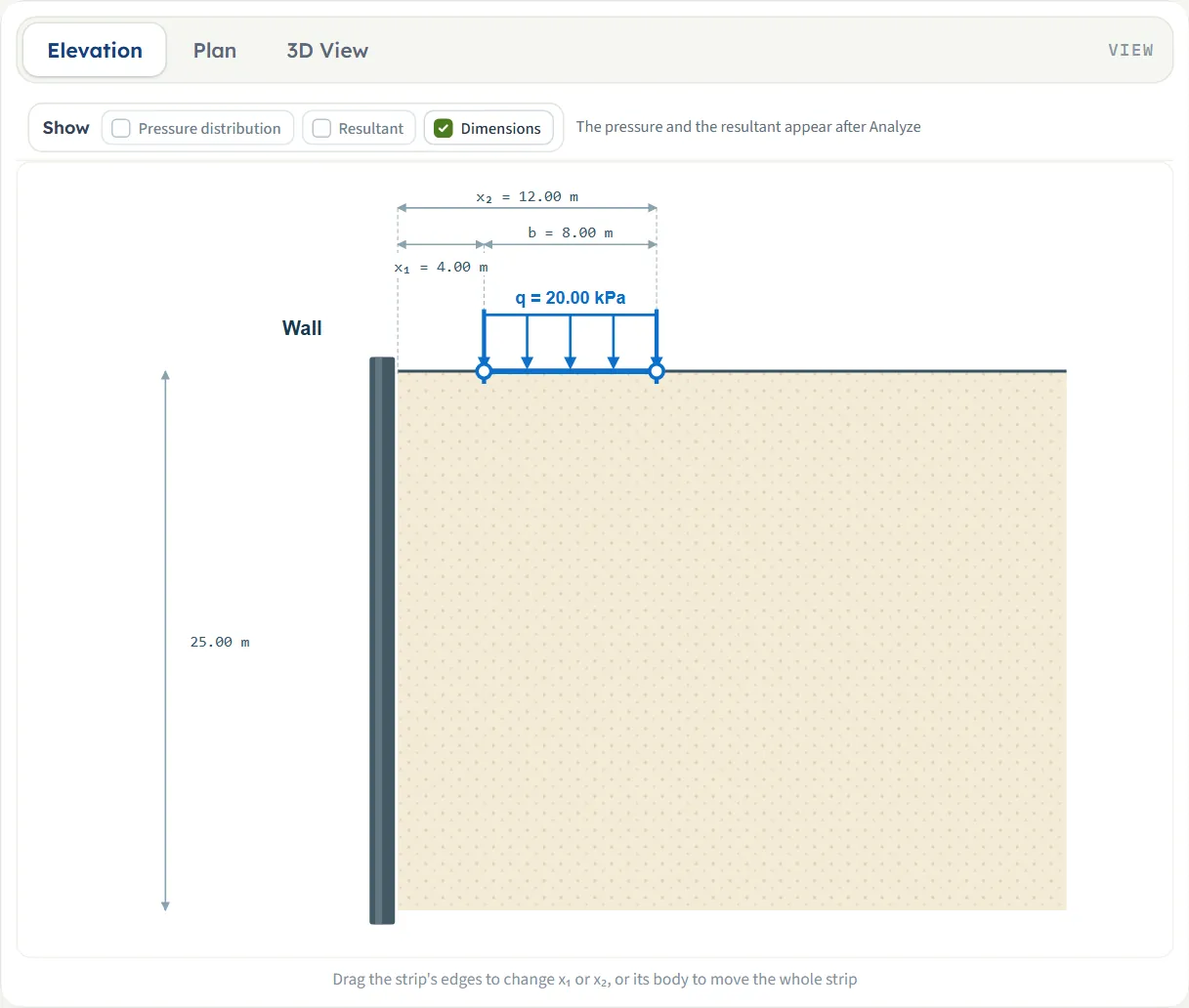
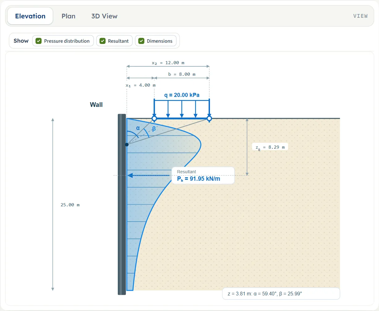
- Elevation shows the wall in section, the strip on the ground with the value of q over its arrows, the pressure diagram on the wall, and the resultant PH with its level zR. The diagram carries the construction of α and β at the depth of the peak pressure, with the values written at the foot of the drawing.
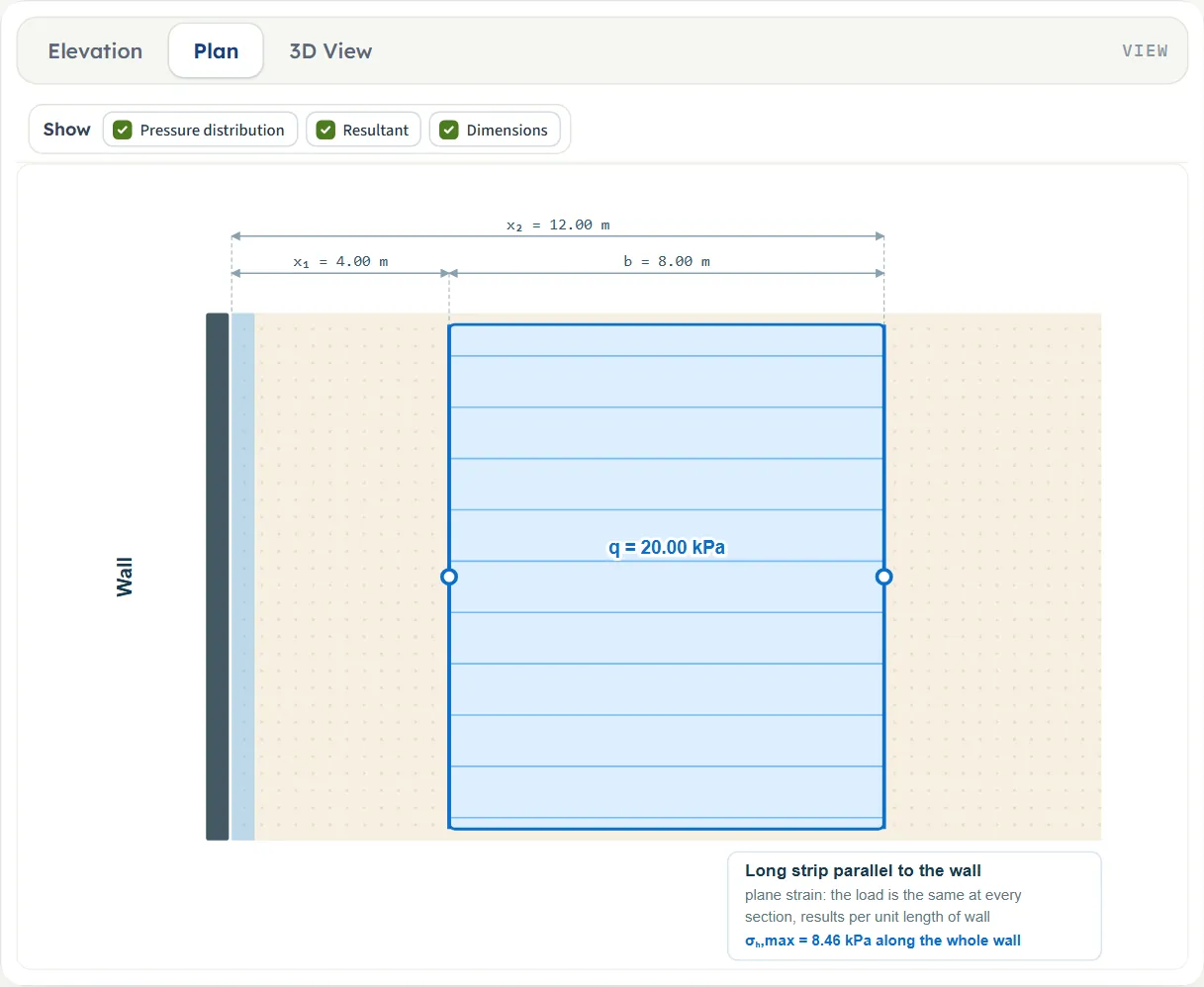
- Plan shows the strip beside the wall seen from above, with the peak pressure along the wall. The module says there: “Long strip parallel to the wall” (plane strain: the load is the same at every section, results per unit length of wall).
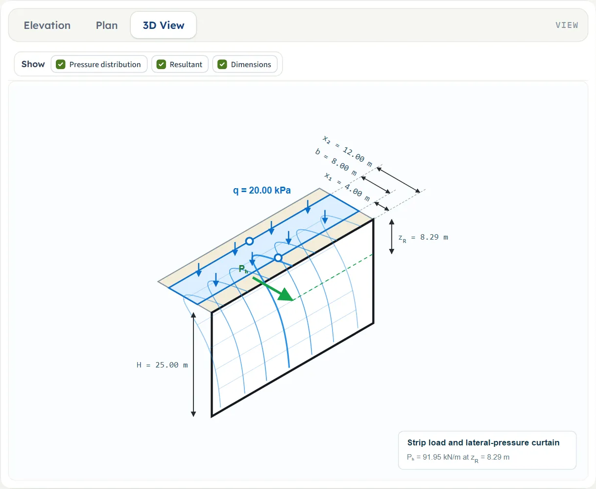
- 3D View shows the strip on the ground and the pressure on the wall as a curtain, with PH at zR.
The Show chips
Above the drawing three chips switch parts of it on and off:
- Pressure distribution: the pressure diagram on the wall, with the angles in the elevation. It is available once the model is analysed; before that the module says “The pressure and the resultant appear after Analyze”.
- Resultant: the resultant arrow and its level. The chip’s hint says it acts in the Elevation and 3D views. It too is available after Analyze.
- Dimensions: the distances, the width and the height. It works at any time, before and after Analyze.
Dragging the strip
Under the drawing the module says: “Drag the strip's edges to change x₁ or x₂, or its body to move the whole strip”. It works in all three views, and the boxes of the Model tab follow as you drag, so the two always agree.
- An edge changes x1 or x2. The edges never pass each other, and the near edge stops at the wall (x1 = 0).
- The body moves the whole strip and keeps its width; it stays on the ground surface and within the extent of the drawing.
- Positions snap to 0.05 of the unit shown (0.05 m, or 0.05 ft in US units). Type the number to set a value more finely.
- After Analyze the strip cannot be dragged: the inputs are locked, and the hint under the drawing is hidden. Edit inputs unlocks the model.
Entering the model, section by section
The Model tab has three sections, Geometry, Strip load and Method. Each opens when you click its title; Next and Back at the foot walk you through them, and the Analyze bar stays at the bottom. The drawing follows every value you type. The tables list each field with its symbol, its unit in the three unit systems (m · ft means m in the two SI systems and ft in US; equal units are merged) and its default, shown in SI · kN.
Geometry
The wall and the place of the strip. The three distances are measured horizontally from the wall, along the ground surface.
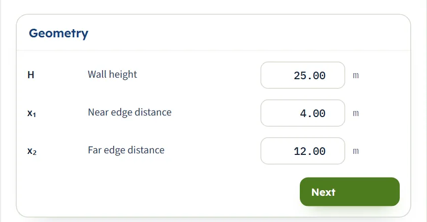
| Field | Symbol | Unit | Default | What to enter |
|---|---|---|---|---|
| Wall height | H | m · ft | 25.00 | Height of the wall, from the ground surface to its base. It must be greater than zero. |
| Near edge distance | x1 | m · ft | 4.00 | Distance from the wall to the near edge of the strip. Zero or more; it must be less than x2. Zero puts the strip against the wall face. |
| Far edge distance | x2 | m · ft | 12.00 | Distance from the wall to the far edge of the strip. It must be greater than x1; the width of the strip is b = x2 − x1. |
Strip load
The load on the strip. It is uniform across the strip and the same along it.
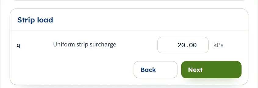
| Field | Symbol | Unit | Default | What to enter |
|---|---|---|---|---|
| Uniform strip surcharge | q | kPa · t/m² · ksf | 20.00 | Load per unit area on the strip, zero or more. The pressure on the wall is proportional to it. |
Method
Two buttons choose how the wall is taken to behave; the note under them says it in a line, and the (?) beside each opens a window with a drawing of the pressure and the formula, with the result of the current inputs by both methods. Choosing the method says more.
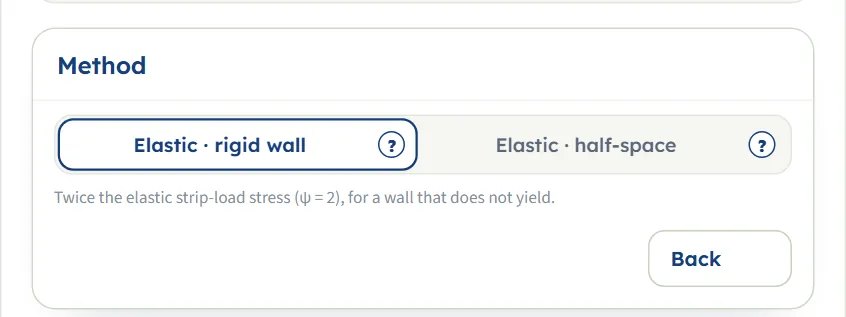
| Choice | Options | Default |
|---|---|---|
| Calculation method | Elastic · rigid wall Elastic · half-space | Elastic · rigid wall |
Units
The unit selector in the header works at any time, before and after Analyze. The boxes are re-written in the new units, and the drawing, the results, the calculations and the report follow. The same example in the three systems:
| Field | SI · kN | SI · tf | US |
|---|---|---|---|
| Wall height | 25.00 m | 25.00 m | 82.02 ft |
| Near edge distance | 4.00 m | 4.00 m | 13.12 ft |
| Far edge distance | 12.00 m | 12.00 m | 39.37 ft |
| Uniform strip surcharge | 20.00 kPa | 2.04 t/m² | 0.4177 ksf |
| Result | SI · kN | SI · tf | US |
|---|---|---|---|
| Resultant force PH | 91.95 kN/m | 9.38 tf/m | 6.30 kip/ft |
| Resultant depth zR | 8.29 m | 8.29 m | 27.19 ft |
| Peak pressure σH,max | 8.46 kPa | 0.8629 t/m² | 0.1767 ksf |
| Depth of peak pressure | 3.81 m | 3.81 m | 12.49 ft |
They are the same answer in other units. In the tf system the force is per metre of wall in tf (1 tf = 9.80665 kN), and the pressure is in t/m².
Choosing the method
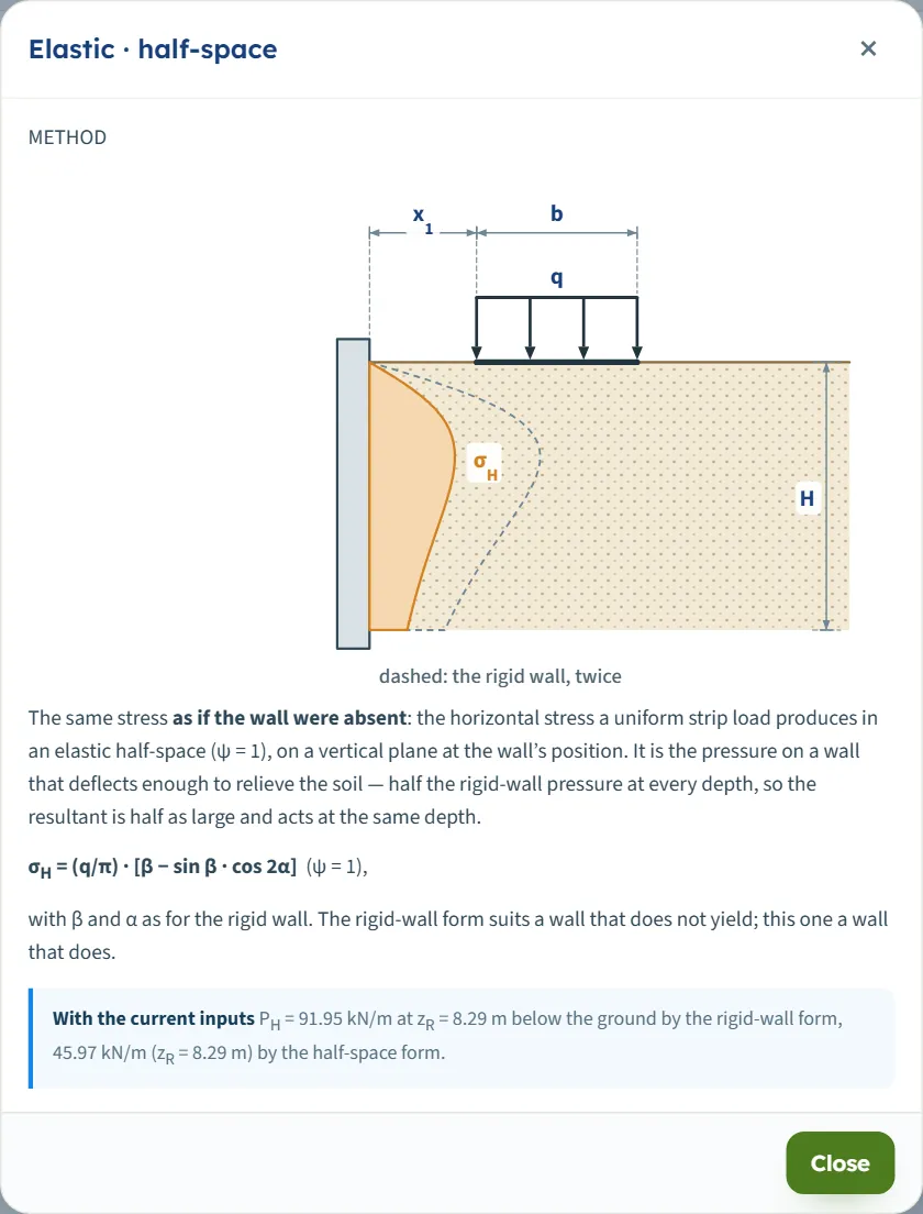
Both methods use the same stress of a strip load on an elastic half-space; they differ in what the wall does to it. They share the angles β and α, so the diagram has the same shape; only its size differs.
| Method | Pressure | ψ | The wall | What it means |
|---|---|---|---|---|
| Elastic · rigid wall (default) | σH = (2q/π) [β − sin β cos 2α] | 2 | Smooth and unyielding | The wall stops the soil at its face from moving horizontally. A mirror-image strip on the other side of the face reproduces that exactly, which is why the stress is doubled (the method of images). |
| Elastic · half-space | σH = (q/π) [β − sin β cos 2α] | 1 | Deflects enough to relieve the soil | The same stress as if the wall were absent, on a vertical plane at the position of the wall. |
The half-space pressure is half the rigid-wall pressure at every depth, so its resultant is half as large and acts at the same depth. For the default example the module gives 45.97 kN/m against 91.95 kN/m, both at 8.29 m below the ground.
Which should I pick?
- Rigid wall is the module’s default. Use it for a wall that does not yield.
- Half-space is for a wall that deflects enough to relieve the soil. It gives the lower of the two pressures.
- Compare. Run both on the same layout and note the two results. The (?) window of either method also prints the result of the current inputs by both forms.
Analyze and read the results
Press Analyze. The bar changes to “Analysed — the lateral pressure calculated” and says: “The inputs are locked. Edit inputs clears the results; the unit system can still be changed.” The Results and Calculations tabs say, until then: “Press Analyze on the Model tab to calculate the lateral pressure.”
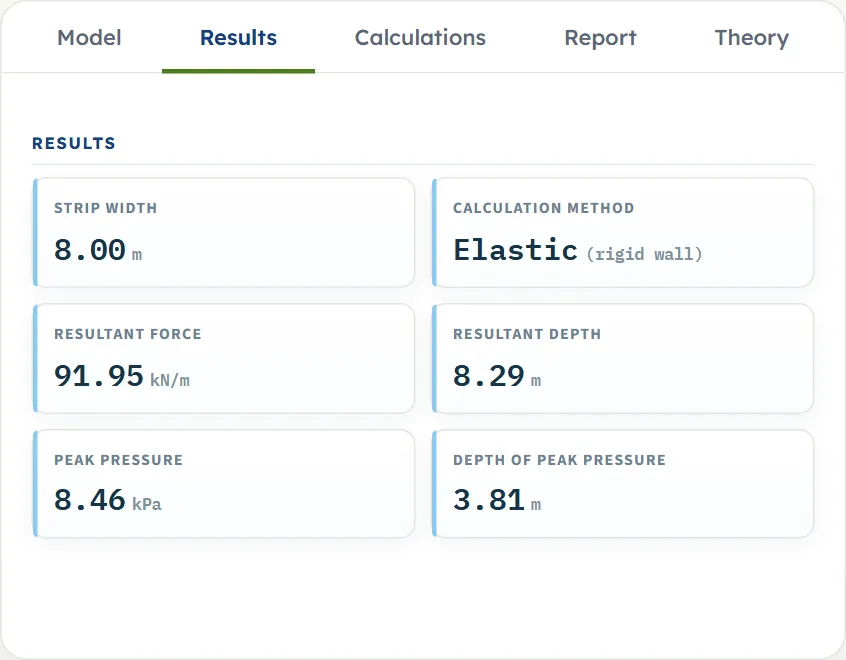
The Results tab shows six cards:
- Strip width: b = x2 − x1.
- Calculation method: Elastic, with “(rigid wall)” or “(half-space)”.
- Resultant force: PH, per unit length of wall (kN/m, tf/m or kip/ft).
- Resultant depth: zR, below the ground surface.
- Peak pressure: the largest ordinate of the pressure diagram, σH,max.
- Depth of peak pressure: where that ordinate is.
For the default example: PH = 91.95 kN/m at zR = 8.29 m, and σH,max = 8.46 kPa at 3.81 m.
How to read the pressure diagram
- It starts at zero at the ground surface when the strip is clear of the wall (x1 > 0), rises to a peak and falls away with depth. In the example the table of the Calculations tab goes from 0.00 kPa at the surface to 8.42 kPa at 4.17 m, and falls to 0.6971 kPa at the base.
- The resultant is the area of that diagram; zR is its centroid, measured down from the ground. The Calculations tab also gives the height above the base (16.71 m in the example).
- The pressure scales with q and the diagram does not depend on the height of the wall: a taller wall adds the lower part of the same diagram, so PH grows and the peak stays where it is.
The Calculations tab and the report
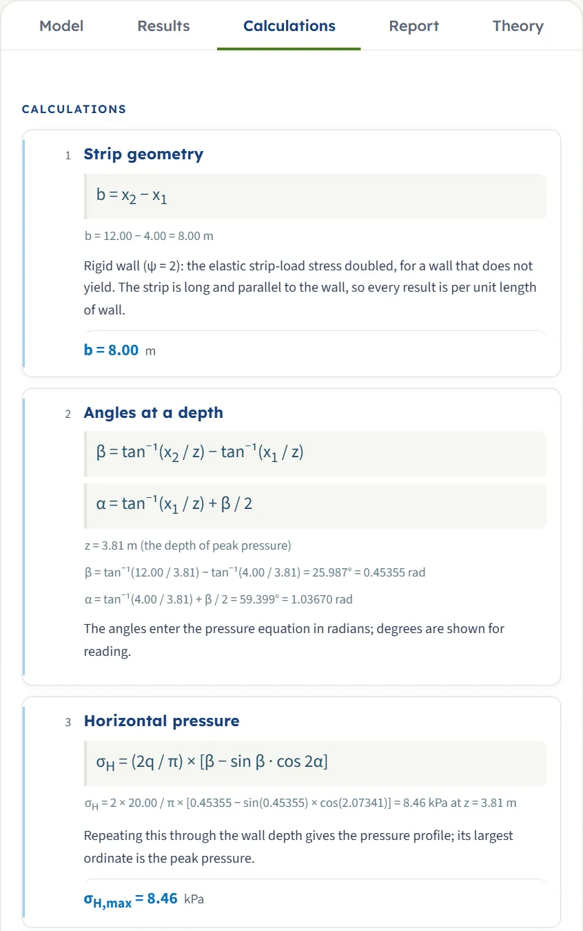
The Calculations tab writes out the working in four numbered steps and a table of the pressure profile:
- Strip geometry: b = x2 − x1, and the method with its ψ.
- Angles at a depth: β and α, in degrees and in radians, worked at the depth of the peak pressure.
- Horizontal pressure: the pressure equation with your numbers, giving σH,max.
- Pressure profile, every H/30: a table of z, β, α and σH at 31 depths from the surface to the base.
- Resultant and its depth: PH = ψ (q/π) H (θ2 − θ1) with θi = tan−1(xi/H), and zR = ∫ z σH dz / PH, below the ground and above the base.
The module says there that both integrals are evaluated numerically to full precision, and that the area also has the exact closed form that is shown as the working. In the example θ1 = tan⁻¹(4.00 / 25.00) = 0.158655 rad and θ2 = tan⁻¹(12.00 / 25.00) = 0.447520 rad, so the closed form gives PH = 91.95 kN/m, as the cards say.
The report
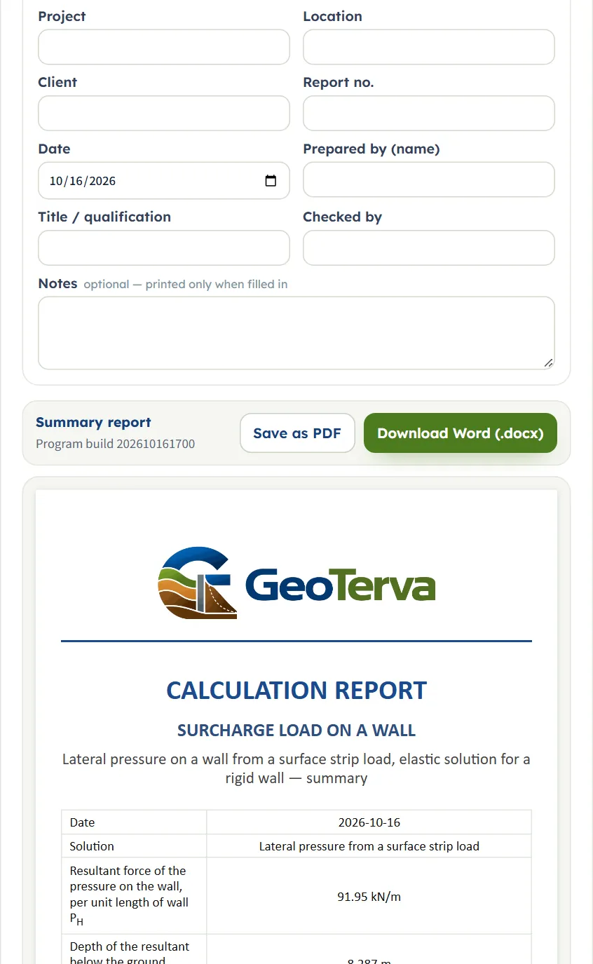
The Report tab turns the same working into a summary report. Fill in the cover (project, location, client, report number, date, prepared by, title or qualification, checked by, notes) and press Save as PDF or Download Word (.docx); the report is made from the analysed model, so press Analyze first. The preview below shows the cover, with the resultant, its depth and the peak pressure, and the whole report. It has six parts: 1 Introduction and scope, 2 Input data (with the three figures: elevation, plan and 3D), 3 Calculation, 4 Results, 5 Summary and 6 References. When the run has a note, the report adds Assumptions and notes after Results and the parts after it move down by one. The units line states the conversion constants. The report prints a little more than the cards: 8.29 m below the ground is 8.287 m in its results table, and the peak pressure is 8.462 kPa.
The Theory tab explains the method in five numbered parts: Strip load on a wall, Pressure at a depth, Resultant and line of action, Worked example and References.
Worked example: the module’s own example
The module opens on this example each time the page is opened, so you can follow the numbers on your own screen.
| Section | Input | Value |
|---|---|---|
| Geometry | Wall height | H = 25.00 m |
| Geometry | Near and far edge | x1 = 4.00 m, x2 = 12.00 m |
| Strip load | Load | q = 20.00 kPa |
| Method | Method | Elastic · rigid wall (ψ = 2) |
Step 1: the strip
The strip is b = 12.00 − 4.00 = 8.00 m wide, from 4.00 m to 12.00 m from the wall.
Step 2: the angles at the depth of the peak
The peak pressure is at z = 3.81 m (the module works at the unrounded depth, 3.8084 m, and shows it as 3.81 m). There β = tan⁻¹(12.00 / 3.81) − tan⁻¹(4.00 / 3.81) = 25.987° = 0.45355 rad and α = tan⁻¹(4.00 / 3.81) + β / 2 = 59.399° = 1.03670 rad. The drawing shows the two rays from that point of the wall to the edges of the strip, with the angles.
Step 3: the pressure
The module prints σH = 2 × 20.00 / π × [0.45355 − sin(0.45355) × cos(2.07341)] = 8.46 kPa at z = 3.81 m. As a check at another depth, take z = 5.00 m, one row of the pressure table: β = 28.720°, α = 53.020°, so σH = 2 × 20 / π × [0.50126 − sin 28.720° × cos 106.040°] = 8.07 kPa, which is the value in the table (5.00 | 28.720 | 53.020 | 8.07).
Step 4: the resultant and its depth
With θ1 = 0.158655 rad and θ2 = 0.447520 rad:
This is the area of the diagram. Its centroid is at zR = 8.29 m below the ground; the Calculations tab says “zR = 8.29 m below the ground (16.71 m above the base)”. The module evaluates zR numerically from the diagram (it also has an exact closed form), and the report prints it as 8.287 m.
How each input changes the answer
Each row below changes one thing (or the two edges together) in the example and runs the module again. The numbers are the results the module gives, so you can reproduce any row. The method is the rigid wall unless the row says otherwise.
| Change | PH (kN/m) | zR (m) | σH,max (kPa) | at z (m) | What happens |
|---|---|---|---|---|---|
| The default example | 91.95 | 8.29 | 8.46 | 3.81 | The reference |
| Half-space method | 45.97 | 8.29 | 4.23 | 3.81 | Exactly half of the rigid-wall values at every depth; zR is the same |
| Wall height 15 m | 79.09 | 6.54 | 8.46 | 3.81 | Less of the diagram: PH and zR both fall (the lower, heavier part is cut off); the peak and its depth do not change |
| Wall height 40 m | 97.68 | 9.62 | 8.46 | 3.81 | More of the diagram: PH grows a little, zR deepens; the peak does not change |
| Strip at the wall face (x1 = 0) | 142.45 | 6.32 | 20.00 | 0.00 | The peak is at the ground surface and equals q; the strip is 12 m wide |
| Strip nearer: x1 = 2, x2 = 10 | 95.71 | 6.72 | 11.53 | 2.33 | The same width, nearer: a higher and shallower peak, a larger PH |
| Strip further: x1 = 8, x2 = 16 | 82.64 | 10.63 | 5.57 | 6.40 | The same width, further away: a lower, deeper peak and a smaller PH |
| Strip further still: x1 = 20, x2 = 28 | 53.22 | 14.06 | 2.76 | 13.60 | Further again: the load acts on the wall much deeper |
| Wider strip: x2 = 20 | 164.28 | 10.01 | 11.53 | 4.66 | The far edge moves out to 20 m: width 16 m, a larger PH |
| Narrower strip: x2 = 6 | 24.47 | 6.12 | 3.32 | 2.81 | A strip 2 m wide: the force falls to about a quarter |
| Strip load q = 40 kPa | 183.90 | 8.29 | 16.92 | 3.81 | Twice the load: twice the pressure and the force; the depths are the same |
| Strip load q = 10 kPa | 45.97 | 8.29 | 4.23 | 3.81 | Half the load: half the pressure and the force |
| Strip load q = 0 | 0.00 | 8.29 | 0.00 | 0.00 | No pressure; the module still reports zR from the geometry |
| Strip at the wall face, half-space | 71.23 | 6.32 | 10.00 | 0.00 | Strip at the wall face by the half-space method: the peak at the surface is q/2 |
Three things stand out. The distance matters as much as the load: moving the same 8 m strip from 4–12 m to 20–28 m takes PH from 91.95 to 53.22 kN/m and zR from 8.29 m to 14.06 m. The width counts: the strip to 20 m gives 164.28 kN/m. The load is a straight proportion: 10, 20 and 40 kPa give 45.97, 91.95 and 183.90 kN/m.
Messages: stops and notes
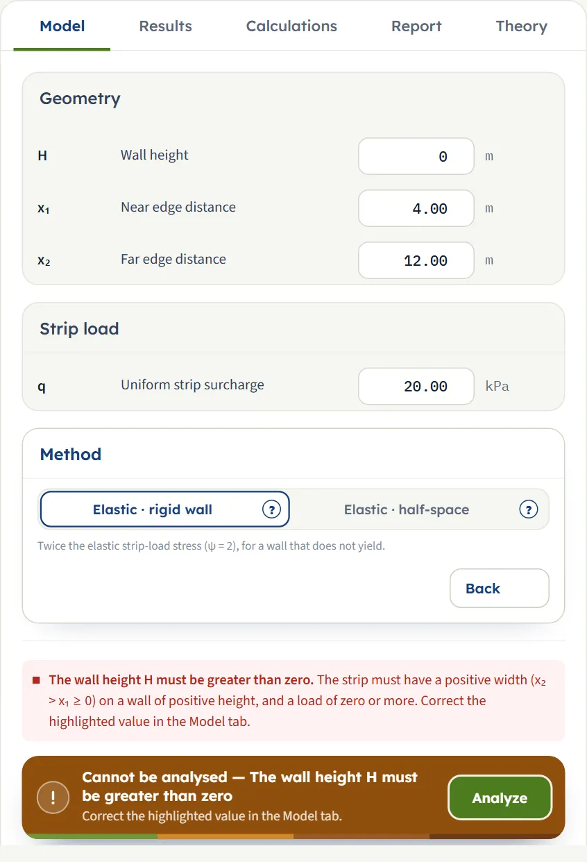
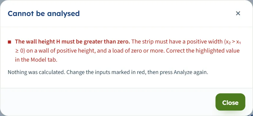
The module says in plain words when something prevents the calculation, and it points to the box to correct. A mistake shows as soon as you type it: a red message appears in the Model tab above the Analyze bar and the bar turns brown and reads “Cannot be analysed”, with the first problem. If you press Analyze anyway a window with the title Cannot be analysed lists the problems; nothing is calculated.
| Kind | When | Message and what to do |
|---|---|---|
| Stop | The wall height is zero, negative or empty | “The wall height H must be greater than zero.” Enter a height above zero. |
| Stop | The near edge is negative or empty | “The near-edge distance x₁ must be zero or more.” Zero puts the strip against the wall. |
| Stop | The far edge is empty | “Enter the far-edge distance x₂.” Fill in x2. |
| Stop | The far edge is not beyond the near edge (equal or less) | “The far edge x₂ must lie beyond the near edge x₁.” The strip must have a width. |
| Stop | The load is negative or empty | “The strip surcharge q must be zero or more.” Enter q of zero or more. |
| Stop | More than one of these at once | The messages are joined: “The wall height H must be greater than zero; The strip surcharge q must be zero or more.” and the window says “Correct the highlighted values in the Model tab.” |
| Note | The strip starts at the wall face (x1 = 0) | “The strip starts at the wall face. At the ground surface the angles take their limits from below (β = 90°, α = 45°), so the pressure there is ψq/2 rather than zero.” The note is shown in the Calculations tab, and the report adds it in Assumptions and notes. The result is valid. |
Every stop is followed by: “The strip must have a positive width (x₂ > x₁ ≥ 0) on a wall of positive height, and a load of zero or more. Correct the highlighted value in the Model tab.” With two or more faults at once the module says “values” (plural). The note about the wall face is the only note this module gives.
Good practice and common mistakes
- Measure x1 and x2 from the wall. They are horizontal distances along the ground surface, from the wall to the two edges of the strip, as the drawing dimensions show.
- Check that the load is a long strip. The module takes the strip as long and parallel to the wall, with the same load at every section. For a load of limited length along the wall use the rectangular areas, and for a single load the point load.
- Choose the method for the wall. The rigid-wall form is twice the half-space form, so the choice changes every pressure and the resultant by a factor of two. Run both when you are unsure how the wall behaves.
- Combine the result with the rest of your wall analysis. The module gives the surcharge component, from the strip alone and with no soil properties; combine it with the earth, water and other actions of your wall analysis.
- Watch the wall height. A taller wall adds the lower part of the same diagram. The force grows more slowly as H increases (79.09 kN/m at 15 m, 91.95 kN/m at 25 m, 97.68 kN/m at 40 m), and the peak does not change.
- Fine-tune by typing. Dragging snaps to 0.05; type the distances you mean.
- Check the units after you switch the system: type values in the units shown beside the boxes.
- Note what you need. The module does not keep the values you type when the page is closed or reloaded; note the layout and the results of each run, or save the report as PDF or Word.
Frequently asked questions
How do I calculate the lateral pressure on a wall from a strip load?
Enter the wall height H, the distances x1 and x2 of the near and far edge of the strip from the wall and the load q, choose the method, and press Analyze. The module gives the resultant PH per unit length of wall, the depth zR at which it acts and the peak pressure, from σH = ψ (q/π) [β − sin β cos 2α]. For the module’s example it gives 91.95 kN/m at 8.29 m.
What is the difference between Elastic · rigid wall and Elastic · half-space?
The rigid-wall method doubles the elastic strip-load stress (ψ = 2) for a wall that does not yield; the half-space method uses the stress as if the wall were absent (ψ = 1), for a wall that deflects enough to relieve the soil. At every depth the half-space pressure is half the rigid-wall pressure, so its resultant is half as large and acts at the same depth: 45.97 kN/m against 91.95 kN/m for the example.
What do x1 and x2 measure?
The horizontal distance from the wall to the near edge (x1) and to the far edge (x2) of the strip, along the ground surface. x2 must be greater than x1, and x1 may be zero. The width of the strip is b = x2 − x1.
Why is the pressure zero at the ground surface?
When the strip is clear of the wall (x1 > 0) the angle it subtends at a point of the wall at the surface is zero, so there is no pressure there. It rises to a peak below the surface, 8.46 kPa at 3.81 m in the example, and falls with depth.
What happens when the strip touches the wall?
With x1 = 0 the angles take their limits at the surface and the pressure there is ψq/2 rather than zero: 20.00 kPa for the rigid wall with q = 20 kPa, and 10.00 kPa by the half-space method. The module gives a note about it, and the result is valid.
Does the result depend on the soil?
No soil properties are asked for. The elastic strip-load solution depends on the geometry and the load only. The module gives the surcharge component; combine it with the earth, water and other actions of your wall analysis.
Does a taller wall change the pressure?
The pressure at a given depth does not depend on the height of the wall, so the peak and its depth stay the same. A taller wall adds the lower part of the diagram, so the resultant grows and acts deeper: 79.09 kN/m at 15 m, 91.95 kN/m at 25 m and 97.68 kN/m at 40 m.
What is the unit of the resultant force?
Force per unit length of wall: kN/m in SI · kN, tf/m in SI · tf and kip/ft in US. The strip is long, so every result is per unit length of the wall.
Can I move the strip with the mouse?
Yes, before Analyze. Drag an edge to change x1 or x2, or the body to move the strip with its width kept. It works in the Elevation, Plan and 3D views and the boxes follow. After Analyze the model is locked; Edit inputs unlocks it.
Why can I not edit the inputs after Analyze?
After a run the inputs are locked, so that the drawing, the results, the calculations and the report all describe the same model. Press Edit inputs to unlock them; the results are cleared. The unit system can still be changed. The workspace guide describes the lock.
Does the module remember my inputs?
No. It opens on its example (a 25 m wall, a 20 kPa strip from 4 m to 12 m, the rigid wall) each time the page is opened. The unit system is remembered.
How do I compare the two methods?
Run the first and note the results, press Edit inputs, choose the other method and run again. The (?) window of each method also prints the resultant of the current inputs by both forms.