

What the module calculates
Line load gives the extra lateral pressure that a long line load on the ground, running parallel to a wall, pushes on the wall. It gives the pressure σH at every depth, the resultant PH per unit length of wall, and the depth zR below the ground at which the resultant acts. With m = x/H and n = z/H, the pressure of the default method is
P is the line load, a force per unit length of the line; x is its distance from the wall; H is the wall height. I0 and I1 are the area and the first moment of the pressure diagram over the height of the wall, written in closed form, so the resultant and its depth are exact. The wall is taken as smooth and unyielding, and the line load is long, so the problem is two-dimensional and every result is per unit length of wall.
What you can describe
- A wall of height H (greater than zero), standing at the edge of the ground surface that carries the load.
- A line load P of zero or more, parallel to the wall, at a distance x of zero or more from it.
- One of two methods: Elastic · rigid wall (the default) and the Terzaghi–NAVFAC chart.
The module draws the load and the pressure diagram in elevation, in plan and in 3D, gives the six numbers of the Results tab, writes out the working, and prepares a PDF or Word report. You can drag the line on the drawing to change its distance from the wall.
What belongs to other modules
- This is the surcharge component only: the extra pressure from this one line. It is added to the earth pressure, the water pressure and the other surcharges in the wall calculation, where you combine them.
- A load that has a width is not a line. A uniform load on a strip parallel to the wall is the Strip load; a concentrated load is the Point load; the other shapes are the Triangular load, the Uniform load, the Area loads and the Ramp load.
Before you start: what you need
Have these ready from your design:
| What | Where it comes from | Notes |
|---|---|---|
| The wall height H | Your design | The height over which the pressure is worked out, from the ground surface to the base of the wall. It must be greater than zero. |
| The line load P | Your design loading | A force per unit length of the line, in kN/m (tf/m or kip/ft in the other systems). Zero or more. A narrow strip of width b carrying a pressure q acts as a line load P = q b when b is small against its distance from the wall. |
| The distance x | Your layout | Measured on the ground, from the face of the wall to the line. Zero or more. A line nearer than 0.30 m is calculated at 0.30 m by the elastic method; see Messages. |
| The method | Your design basis | Elastic · rigid wall, or the Terzaghi–NAVFAC chart. The two give the same result once x is beyond 0.4H. |
The module needs no soil properties: the pressure follows from the geometry and the load alone.
Quick start in seven steps
- Open the module and choose the units
Open Line load from the Surcharge Loads family. Pick SI · kN, SI · tf or US in the header; you can change it at any time. Open Line load.
- Enter the geometry
In Geometry, type the wall height H and the distance x from the wall to the line.
- Enter the line load
In Line load, type the load P per unit length of the line.
- Choose the method
In Method, pick Elastic · rigid wall or Terzaghi–NAVFAC chart. The (?) beside each opens a window with a sketch of what it assumes.
- Press Analyze
Press Analyze at the foot of the Model tab. The bar reads Analysed, the inputs lock, and the pressure and the resultant appear on the drawing.
- Read the answer
The Results tab gives six numbers: the distance ratio, the method (or case), the resultant PH, its depth zR, the peak pressure and its depth. Elevation, Plan and 3D View change the view.
- Take the working and the report
The Calculations tab shows the three steps with your numbers and the pressure at every H/30. The Report tab saves a PDF or a Word file.
The screen: three views and a line you can drag
The layout is the one every GeoTerva module shares, described in the workspace guide. For this module the drawing has three views, chosen with the buttons above it:
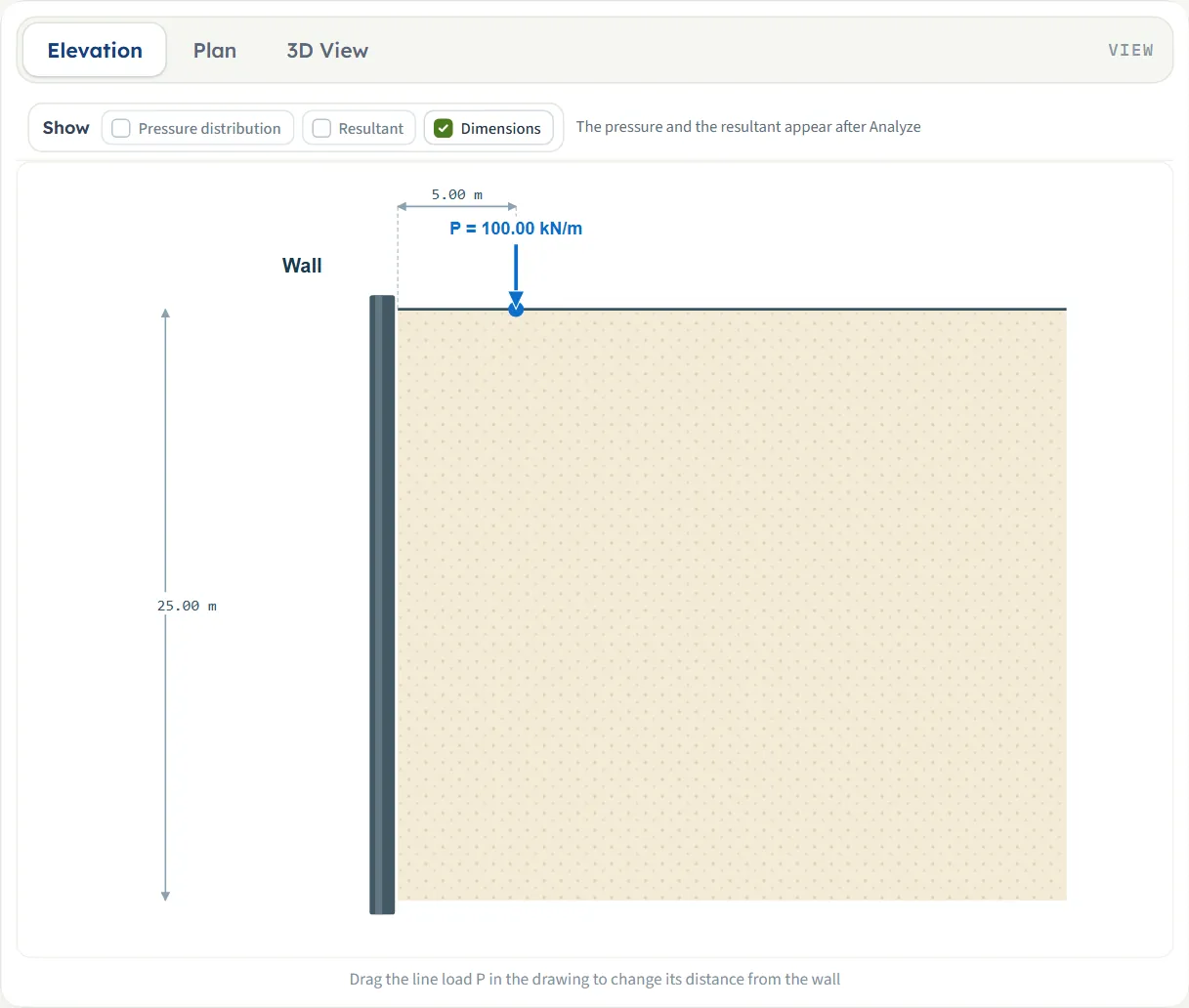
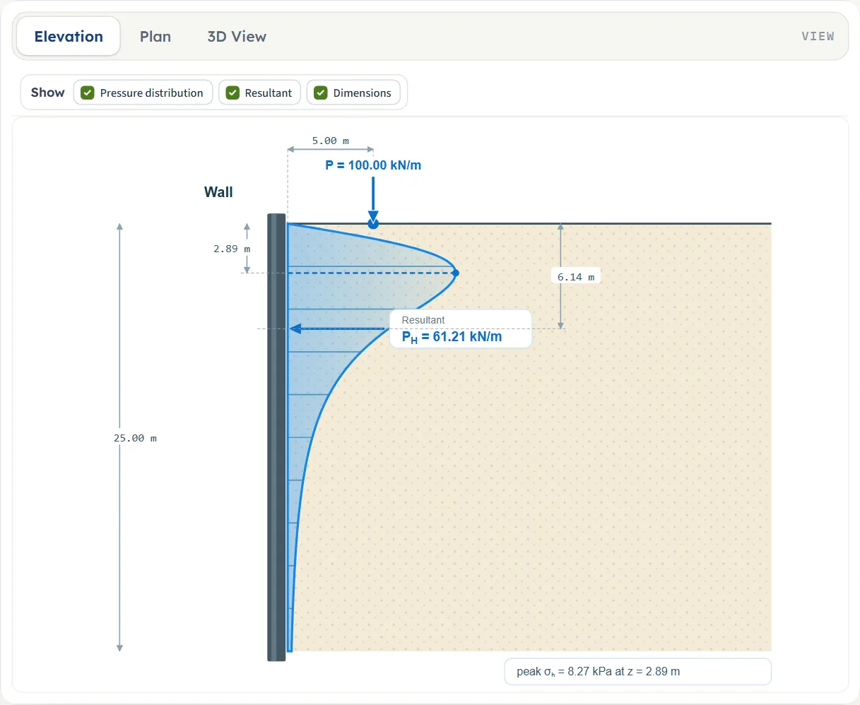
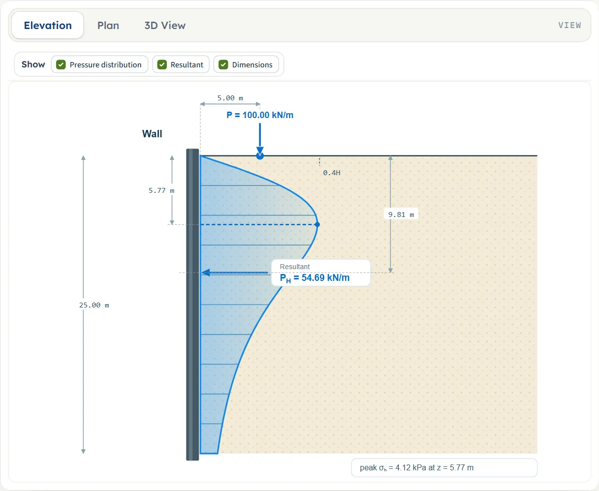
- Elevation is a section through the wall and the ground: the wall, the soil, the line load as an arrow with its value, the distance x and the wall height H. After Analyze it adds the pressure diagram on the wall, with ordinates at every tenth of the height, a dashed line at the peak with its depth, the resultant PH acting on the wall with its depth zR, and a note with the peak pressure.
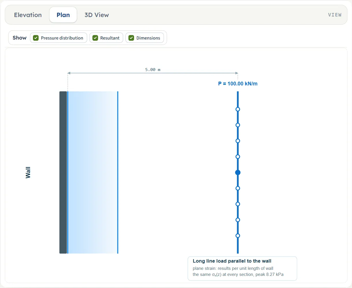
- Plan looks down on the ground. The line is drawn parallel to the wall, with rings along it and a filled dot in the middle, and its distance from the wall. After Analyze a band along the wall shows that the same pressure acts at every section, and a note at the foot of the drawing says the load is long, the problem is plane strain and the results are per unit length of wall.
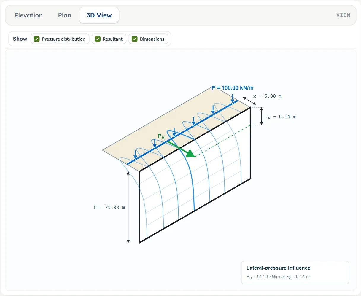
- 3D View shows the wall, the ground behind it and the line with a row of arrows. After Analyze the pressure is drawn as a curtain on the wall face, with the resultant PH as an arrow at its depth and the dimensions H, x and zR.
The Show chips
Above the drawing a Show bar has three chips. Pressure distribution and Resultant are available after Analyze; until then they are greyed and the bar says “The pressure and the resultant appear after Analyze”. Dimensions can be switched at any time: it shows or hides the dimension lines with their values. Pressure distribution switches the pressure diagram, its peak and the note with the peak; Resultant switches the resultant arrow, its label and its depth, in the elevation and the 3D view (a plan has no place for a resultant).
Dragging the line
Before you analyse you can move the line instead of typing: press the load arrow (or, in the plan, the line; in the 3D view, the line or one of its arrows) and drag it sideways. The distance box follows the drawing and the drawing follows the box. The distance moves in steps of 0.05 (m or ft, as shown), cannot go below zero, and stops at the edge of the drawing. The note under the drawing says “Drag the line load P in the drawing to change its distance from the wall”. After Analyze the inputs are locked, the drag is off and that note is hidden; Edit inputs gives it back.
Entering the model, section by section
The Model tab has three sections. Each opens when you click its title; Next and Back at the foot walk you through them, and Analyze waits below the last one. The tables list every field with its symbol, the unit in each unit system and its default. Where a unit is shown twice or three times, such as m · ft, the units are those of SI · kN, SI · tf and US in turn, and equal ones are merged. Defaults are shown in SI; in SI · tf the line-load box shows 10.20 tf/m, and in US the boxes show 82.02 ft, 16.40 ft and 6.85 kip/ft for the same wall and load.
Geometry
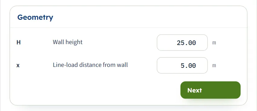
Two numbers: the height of the wall and the distance of the line from it.
| Field | Symbol | Unit | Default | What to enter |
|---|---|---|---|---|
| Wall height | H | m · ft | 25 | The height of the wall over which the pressure is worked out, from the ground surface to the base. It must be greater than zero; a blank or zero box stops the analysis. |
| Line-load distance from wall | x | m · ft | 5 | The distance on the ground from the wall to the line, zero or more. With the elastic method a distance below 0.30 m (0.9843 ft) is calculated at 0.30 m and the module says so. With the chart method a distance within 0.4H gives the same result. |
Line load
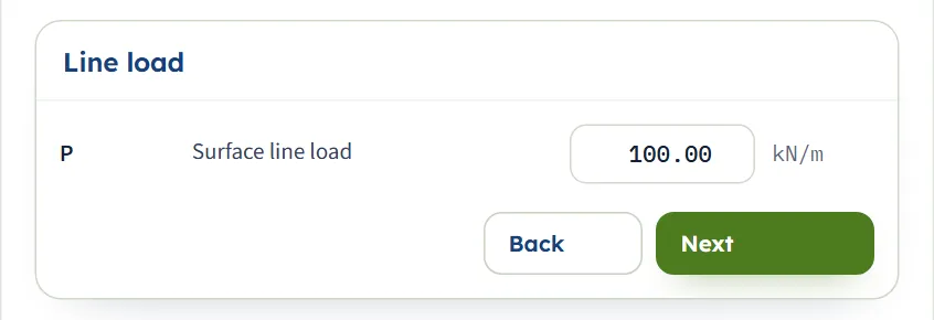
One number: the load per unit length of the line.
| Field | Symbol | Unit | Default | What to enter |
|---|---|---|---|---|
| Surface line load | P | kN/m · tf/m · kip/ft | 100 | The force per unit length of the line, zero or more. The pressure and the resultant are proportional to it; zero gives zero pressure. |
Method
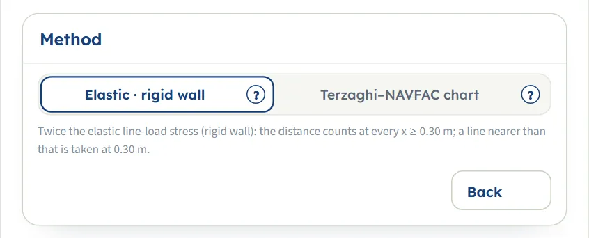
Two buttons choose the solution; each has a (?) that opens a help window. A line under the buttons says what the method assumes, and it follows the unit system.
| Choice | Options | Default |
|---|---|---|
| Calculation method | Elastic · rigid wall Terzaghi–NAVFAC chart | Elastic · rigid wall |
Choosing the method
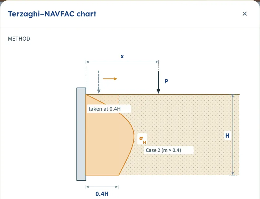
Both methods use the same equation once the line is beyond 0.4 wall heights from the wall (m > 0.4). They differ for a line that is closer.
| Method | Pressure σH | Closer than m = 0.4 | Resultant and depth |
|---|---|---|---|
| Elastic · rigid wall (the default) | (4P / πH) · m² n / (m² + n²)² at every distance | The distance counts at every x of 0.30 m or more. The pressure peaks at n = m/√3, that is z = x/√3, and grows without limit as the line reaches the wall; a line nearer than 0.30 m is calculated at 0.30 m. | PH = P · (2/π) / (1 + m²), zR = H · I1 / I0, with I1 = (2/π) [m tan⁻¹(1/m) − m² / (1 + m²)] |
| Terzaghi–NAVFAC chart | Case 2 (m > 0.4): the same equation. Case 1 (m ≤ 0.4): σH = (P / H) · 0.203 n / (0.16 + n²)² | The line is taken as if it stood at m = 0.4, so its distance has no effect while x ≤ 0.4H. The peak is at n = 0.4/√3. | Case 1: PH = 0.5469 P (from I0 = 0.1015 (1/0.16 − 1/1.16)), zR = H · I1 / I0 with I1 = 0.203 [tan⁻¹(2.5)/0.8 − 1/2.32] |
How far apart the two methods are
The table gives the module’s own results for the example wall (H = 25 m, P = 100 kN/m) as the line moves away from the wall.
| Distance x | Elastic PH | Elastic zR | Chart PH | Chart zR |
|---|---|---|---|---|
| 0.1 m (0.004H); elastic at 0.30 m | 63.65 | 0.4641 | 54.69 | 9.81 |
| 1 m (0.04H) | 63.56 | 1.49 | 54.69 | 9.81 |
| 2 m (0.08H) | 63.26 | 2.84 | 54.69 | 9.81 |
| 5 m (0.2H), the example | 61.21 | 6.14 | 54.69 | 9.81 |
| 7.5 m (0.3H) | 58.41 | 8.21 | 54.69 | 9.81 |
| 10 m (0.4H); chart still Case 1 | 54.88 | 9.81 | 54.69 | 9.81 |
| 12.5 m (0.5H); the methods agree from here | 50.93 | 11.05 | 50.93 | 11.05 |
| 15 m (0.6H) | 46.81 | 12.02 | 46.81 | 12.02 |
| 25 m (H) | 31.83 | 14.27 | 31.83 | 14.27 |
| 50 m (2H); peak at the base | 12.73 | 15.91 | 12.73 | 15.91 |
Inside 0.4H the chart result does not move: PH stays at 54.69 kN/m and zR at 9.81 m, while the elastic resultant rises towards 2P/π = 63.7 kN/m and its depth shrinks towards the wall top. The peak pressure differs much more than the resultant: at 1 m the elastic peak is 41.35 kPa and the chart peak 4.12 kPa.
The (?) windows
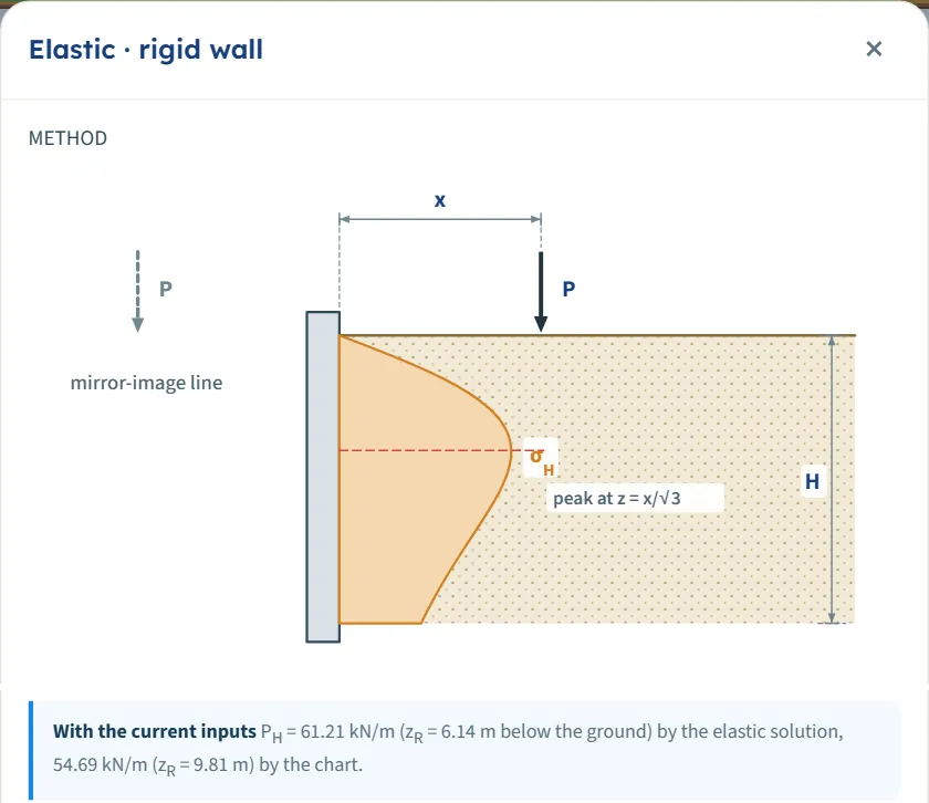
The (?) beside each method opens a window with a sketch of the wall, the line, the pressure diagram and its peak, the equations, and a line headed With the current inputs that gives PH and zR for your H, x and P by both methods side by side (61.21 kN/m at 6.14 m by the elastic solution and 54.69 kN/m at 9.81 m by the chart, for the example). Reading a window changes nothing in the model.
Which should I pick?
- Start with the default, Elastic · rigid wall. The distance counts at every x, so you see what moving the line does, and it needs nothing but H, x and P.
- Use the Terzaghi–NAVFAC chart when your design basis is that chart. Its result is the same as the elastic one beyond 0.4H and is held at the m = 0.4 values inside it.
- Compare when the line is close. Inside 0.4H the two methods give different pressures and depths; run both (Edit inputs between runs) and keep the one your design basis calls for.
- Beyond 0.4H the choice does not matter: the two give the same numbers.
Analyze and read the results
Press Analyze. The bar changes to Analysed — the lateral pressure calculated and says “The inputs are locked. Edit inputs clears the results; the unit system can still be changed.” The Results tab shows six cards, and the drawing now carries the pressure and the resultant.
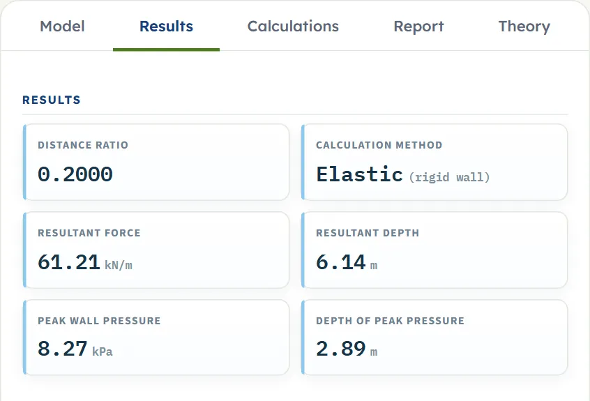
| Card | What it is | The example |
|---|---|---|
| Distance ratio m | The distance of the line in wall heights, x / H. If the line is nearer than 0.30 m, the card shows the ratio as calculated and a line under it gives the ratio as entered. | 0.2000 |
| Calculation method, or Calculation case | For the elastic method: Elastic (rigid wall), or Elastic (at x min) when the line was moved out to 0.30 m. For the chart: Case 1 (m ≤ 0.4) or Case 2 (m > 0.4). | Elastic (rigid wall) |
| Resultant force PH | The area of the pressure diagram over the height of the wall, per unit length of wall. | 61.21 kN/m |
| Resultant depth zR | The depth below the ground at which PH acts. The calculation also gives its height above the base, H − zR. | 6.14 m |
| Peak wall pressure σH,max | The largest pressure on the wall. | 8.27 kPa |
| Depth of peak pressure | The depth at which that pressure acts. | 2.89 m |
Using the numbers
- The pressure diagram is not a rectangle or a triangle but a curve that starts at zero at the ground, peaks and dies away with depth. In the wall calculation add it, point by point or as the resultant PH at zR, to the earth-pressure and water-pressure diagrams.
- PH is a force per unit length of wall. P is a force per unit length of the line, and for a line parallel to the wall these are the same length.
- The peak of the elastic diagram is at z = x/√3 below the ground, unless that is deeper than the wall, in which case the peak is at the base: with x = 50 m the module gives a peak depth of 25.00 m, the wall height.
- The module supplies a lateral action to combine with the other pressures in your wall calculation.
- Changing the unit system after Analyze re-states the cards, the drawing and the report without a new run. Edit inputs unlocks the model and clears the results.
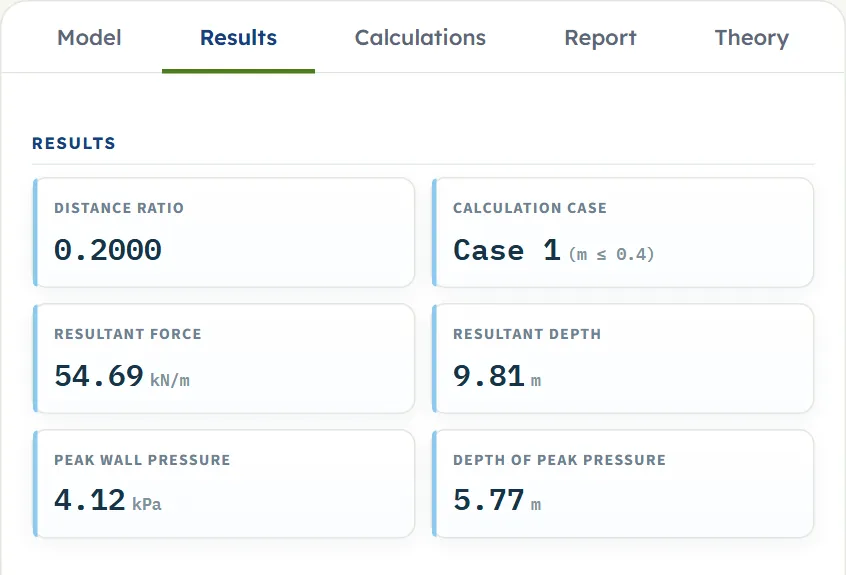
With the Terzaghi–NAVFAC chart the second card reads Calculation case and gives Case 1 (m ≤ 0.4) or Case 2 (m > 0.4), and the elevation marks 0.4H on the ground line.
The Calculations tab and the report
The Calculations tab writes out the working in three numbered steps, each with its equation, the equation with your numbers, a short note and the result:
- Distance ratio — m = x / H with your numbers. For the elastic method a note says that one equation holds for every distance; for the chart it says which case governs, and when the elastic line was moved out to 0.30 m it shows both ratios. The result: m.
- Pressure at a depth — n = z / H at the depth of the peak, the equation for σH and the peak pressure with its depth, followed by a table of z, n and σH at every H/30 (31 rows, from the ground to the base).
- Resultant and its depth — PH = ∫ σH dz = P · I0 and zR = H · I1 / I0, the closed forms of I0 and I1, their values, and the results with the height of the resultant above the base.
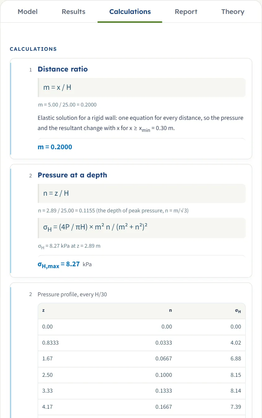
Before Analyze the tab says “Press Analyze on the Model tab to calculate the lateral pressure.” A caution of the run is printed at the end of the working.
The report
In the Report tab fill in the cover (project, location, client, report number, date, prepared by, title, checked by, and optional notes). The cover details are kept in this browser. After Analyze, Save as PDF and Download Word (.docx) are available; before it they are greyed out. The preview below the buttons is the report itself.
The report has six parts: 1 Introduction and scope, 2 Input data, 3 Calculation (one part for each of the three steps), 4 Results, 5 Summary and 6 References. When the run has a caution, as when the line was moved out to 0.30 m, an Assumptions and notes part follows the results and the last two parts move down by one. The report carries the elevation, the plan and the 3D drawing, and states the units with the conversion constants.

The Theory tab has five sections: Line load on a wall, The two methods, Resultant and line of action (with a table of both methods against the distance of the line), Worked example, and References.
Worked example: the module’s own example
The module opens on this example, so you can follow the numbers on your own screen.
| Section | Input | Value |
|---|---|---|
| Geometry | Wall height, distance of the line | H = 25 m, x = 5 m |
| Line load | Load | P = 100 kN/m |
| Method | Method | Elastic · rigid wall |
Step 1: the distance ratio
m = x / H = 5.00 / 25.00 = 0.2000. The line is beyond 0.30 m, so it is calculated where it stands.
Step 2: the peak of the pressure
The peak is at n = m/√3 = 0.2000/1.7321 = 0.1155, that is z = 0.1155 × 25 = 2.89 m. There the pressure is
The same equation at z = 5 m (n = 0.2) gives 5.093 × 0.008 / 0.0064 = 6.37 kPa, the value in the table of the Calculations tab at 5.00 m.
Step 3: the resultant and its depth
I0 = (2/π) / (1 + 0.2000²) = 0.63662 / 1.04 = 0.61213, so PH = 100 × 0.61213 = 61.21 kN/m. I1 = (2/π) [0.2 × tan⁻¹(5) − 0.04/1.04] = 0.63662 × (0.27468 − 0.03846) = 0.15038, so
These are the six numbers of the Results tab and the three steps of the Calculations tab.
The same wall by the chart
Choose Terzaghi–NAVFAC chart (after Edit inputs) and analyse again. m = 0.2 is not above 0.4, so Case 1 governs: the line is taken as if it stood at m = 0.4. I0 = 0.1015 (1/0.16 − 1/1.16) = 0.54688, so PH = 54.69 kN/m; I1 = 0.203 [tan⁻¹(2.5)/0.8 − 1/2.32] = 0.21454, so zR = 25 × 0.21454 / 0.54688 = 9.81 m. The peak is at z = 0.4 × 25/√3 = 5.77 m, where σH = 4.12 kPa.
A smaller wall, a nearer line
For H = 6 m, x = 2 m and P = 40 kN/m, m = 0.3333. By the elastic method I0 = (2/π) / (1 + 1/9) = 0.57296, so PH = 40 × 0.57296 = 22.92 kN/m, and I1 = 0.63662 × (⅓ tan⁻¹(3) − 0.1) = 0.20139 gives zR = 6 × 0.20139 / 0.57296 = 2.11 m; the peak is 8.27 kPa at 1.15 m. By the chart (m ≤ 0.4, Case 1) the module gives PH = 21.88 kN/m at 2.35 m, with a peak of 6.87 kPa at 1.39 m.
How each input changes the answer
Each row below changes one thing in the example (H = 25 m, x = 5 m, P = 100 kN/m, elastic) and runs the module again. The numbers are the ones the module gives, in the units of SI · kN, so you can reproduce any row. The four columns are the resultant PH in kN/m, its depth zR in m, the peak pressure σH,max in kPa and its depth in m.
| Change | PH (kN/m) | zR (m) | σH,max (kPa) | Peak depth (m) |
|---|---|---|---|---|
| The default example: H = 25 m, x = 5 m, P = 100 kN/m, elastic | 61.21 | 6.14 | 8.27 | 2.89 |
| H = 15 m | 57.30 | 5.27 | 8.27 | 2.89 |
| H = 20 m | 59.92 | 5.79 | 8.27 | 2.89 |
| H = 30 m | 61.94 | 6.39 | 8.27 | 2.89 |
| H = 40 m | 62.68 | 6.72 | 8.27 | 2.89 |
| x = 1 m | 63.56 | 1.49 | 41.35 | 0.5774 |
| x = 2 m | 63.26 | 2.84 | 20.67 | 1.15 |
| x = 7.5 m | 58.41 | 8.21 | 5.51 | 4.33 |
| x = 15 m | 46.81 | 12.02 | 2.76 | 8.66 |
| x = 25 m | 31.83 | 14.27 | 1.65 | 14.43 |
| x = 0.1 m (m = 0.0120, calculated at 0.30 m) | 63.65 | 0.4641 | 137.83 | 0.1732 |
| P = 50 kN/m | 30.61 | 6.14 | 4.13 | 2.89 |
| P = 200 kN/m | 122.43 | 6.14 | 16.54 | 2.89 |
| P = 0 | 0.00 | 6.14 | 0.00 | 2.89 |
| Chart method | 54.69 | 9.81 | 4.12 | 5.77 |
| Chart, H = 15 m | 54.69 | 5.88 | 6.87 | 3.46 |
| Chart, H = 40 m | 54.69 | 15.69 | 2.58 | 9.24 |
| Chart, P = 200 kN/m | 109.38 | 9.81 | 8.24 | 5.77 |
- Wall height. A lower wall cuts off more of the tail of the diagram, so PH falls; a higher wall adds a little and PH approaches 2P/π = 63.7 kN/m. The peak does not change.
- Distance. A nearer line gives a sharp, shallow peak (five times higher at 1 m than at 5 m) and a shallow resultant; a farther line gives a lower, deeper, broader diagram. At 0.1 m the line is calculated at 0.30 m, with a caution.
- Load. The pressure and the resultant are proportional to P; the depths do not change. With P = 0 the pressure and the resultant are zero, and the depths are those of the geometry.
- Chart. Case 1 holds the distance out of the result: a lower peak, a deeper resultant, PH = 0.5469 P whatever H is, and the depths follow H.
The pattern follows the formulas: PH and the pressure are proportional to P; the elastic peak, σH = 9P / (4√3 π x) at z = x/√3, depends on the distance and not on the wall height (while the peak lies above the base of the wall; 41.35, 20.67 and 8.27 kPa at 1, 2 and 5 m); and PH falls as the line moves away, from about 2P/π at the wall.
Messages: stops and cautions
The module tells you in plain words when something prevents the calculation and when a result needs care. There are two kinds.
A stop: nothing is calculated
The module checks the three numbers it needs. When one cannot be used it stops:
- A message appears in the Model tab above the Analyze bar, and the bar turns brown and reads Cannot be analysed, followed by the message.
- If you press Analyze, a window titled Cannot be analysed gives the message and says “Nothing was calculated. Change the inputs marked in red, then press Analyze again.”
- The Results tab says “Not calculated — see the Model tab.”, the Calculations tab shows the message, and the drawings say “Not calculated — correct the highlighted input in the Model tab”.

| Kind | When | Message and what to do |
|---|---|---|
| Stop | The wall height is zero, negative or empty | “The wall height H must be greater than zero.” Enter a height above zero. |
| Stop | The line-load distance is negative or empty | “The line-load distance x must be zero or more.” Enter zero or a positive distance. |
| Stop | The line load is negative or empty | “The line load P must be zero or more.” Enter zero or a positive load. |
Every stop continues with the same sentences: “A zero or negative wall height makes m and n undefined; a negative distance or load, or an empty box, has no meaning here. Correct the highlighted value in the Model tab.” When more than one value is wrong the messages are joined in one stop, for example “The wall height H must be greater than zero; The line-load distance x must be zero or more; The line load P must be zero or more.” The message names the value that has to change.
A caution: the line is nearer than the least distance
With the Elastic · rigid wall method the pressure peak grows without limit as the line reaches the wall. A line nearer than 0.30 m (0.9843 ft in US) is therefore calculated at 0.30 m, and the module says so. A distance of exactly 0.30 m is calculated as entered. The chart method has no such limit, because it holds the line at 0.4H from the wall inside that distance.
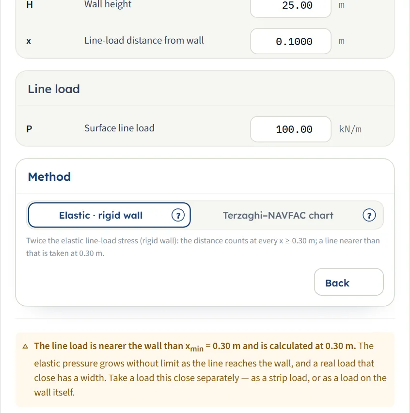
| Kind | When | Message and what to do |
|---|---|---|
| Caution | Elastic method and x below 0.30 m | “The line load is nearer the wall than xmin = 0.30 m and is calculated at 0.30 m. The elastic pressure grows without limit as the line reaches the wall, and a real load that close has a width. Take a load this close separately — as a strip load, or as a load on the wall itself.” |
The caution stays in the Model tab and is printed at the end of the Calculations tab; the report adds an Assumptions and notes part. On the Results tab the first card shows the ratio as calculated, with a line “x/H = … as entered · calculated at x min” under it, and the second card reads Elastic (at x min). For the example wall with the line at 0.1 m the module gives PH = 63.65 kN/m at 0.4641 m and a peak of 137.83 kPa at 0.1732 m, the same as at 0.30 m.
Good practice and common mistakes
- Use this module for a load that is narrow. A line is a load whose width is small against its distance from the wall. For a load with a width, the Strip load module takes the width into account.
- Enter P per unit length of the line, in kN/m, not as a total force. For a narrow strip of width b carrying q, use P = q b.
- Measure x on the ground from the face of the wall to the line, the distance drawn in the elevation.
- Read PH per unit length of wall. Multiply by a length of wall only when you need a total force on that length.
- Add the result to the other pressures. σH is the surcharge component of this one line; the wall calculation combines it with the earth pressure, the water pressure and the other loads.
- Run both methods when the line is within 0.4H of the wall and keep the one your design basis calls for. Beyond 0.4H they agree.
- Watch the peak close to the wall. The elastic peak grows as 1/x: the module gives 41.35 kPa at 1 m and 137.83 kPa at 0.30 m for the example load. A line that close has a width: see the caution above.
- Note your values. The module opens on its example every time and does not keep what you typed; the report is the record of an analysis.
- Check the units after switching the system: type values in the units shown beside the boxes.
Frequently asked questions
How is the lateral pressure from a line load calculated?
For a long line load P parallel to a wall of height H, at a distance x from it, with m = x/H and n = z/H, the elastic solution for a rigid wall gives σH = (4P / πH) m² n / (m² + n²)² at every depth. The resultant PH = P · (2/π) / (1 + m²) is the area of the diagram over the height of the wall. For the module’s example it is 61.21 kN/m, acting 6.14 m below the ground.
Why is the elastic stress doubled?
A smooth, unyielding wall stops the soil at its face from moving horizontally. That doubles the horizontal stress of the elastic half-space, and a mirror-image line load on the far side of the wall face reproduces it exactly (the method of images). The module’s help window for the method draws the mirror-image line.
Where is the peak pressure, and how large is it?
For the elastic method the peak is at z = x/√3 below the ground and equals 9P / (4√3 π x), which does not depend on the wall height. The module gives 8.27 kPa at 2.89 m for the example. If x/√3 is deeper than the wall, the peak is at the base of the wall. For the chart method inside 0.4H the peak is at 0.4H/√3.
What is the difference between the elastic method and the Terzaghi–NAVFAC chart?
They use the same equation when the line is beyond 0.4 wall heights from the wall. Inside that distance the chart takes the line as if it stood at m = 0.4, so its distance has no effect and the resultant stays at 0.5469 P; the elastic method lets the distance count, so a nearer line gives a higher, shallower peak. For the example the two give 61.21 and 54.69 kN/m.
What is the least distance, 0.30 m?
With the elastic method the pressure peak grows without limit as the line reaches the wall, while the resultant stays finite. A line nearer than 0.30 m is calculated at 0.30 m and the module cautions you; a real load that close has a width, and the caution suggests a strip load or a load on the wall itself. The chart method has no such limit.
Are the results per metre?
Yes. The line load is long, so the problem is two-dimensional (plane strain): P is a force per unit length of the line, and PH is a force per unit length of wall. The same pressure acts at every section along the wall.
Does the result include the earth pressure and the water pressure?
No. The result is the surcharge component of this one line load. You add it to the earth-pressure and water-pressure diagrams, and to the other surcharges, in the wall calculation.
What values does the module accept?
The wall height must be greater than zero, the distance of the line zero or more and the line load zero or more. Anything else, or an empty box, stops the analysis with a message that names the value.
Can I drag the line on the drawing?
Yes, before you analyse. Drag the load arrow in the elevation, the line in the plan or the line in the 3D view; the distance box follows, in steps of 0.05 (m or ft). After Analyze the inputs are locked and the drag is off until you press Edit inputs.
Which units does it use, and what are the units of the answer?
SI · kN, SI · tf or US, switchable in the header at any time, even after Analyze. The pressure is in kPa, t/m² or ksf, the resultant per unit length in kN/m, tf/m or kip/ft, and the depths in m or ft.
Does the module remember my inputs?
No. It opens on its example (25 m wall, 100 kN/m at 5 m, elastic) each time the page is opened. The report cover details you type are kept in the browser, and the unit system is remembered.
What does the report contain?
A cover with your project details and a summary, then six parts: introduction and scope, input data, the calculation step by step, results, summary and references, with the elevation, plan and 3D drawings. A caution of the run adds an Assumptions and notes part. It is saved as a PDF or a Word file after Analyze.