

What the module calculates
Area loads gives the extra lateral pressure on a wall from one or more rectangular loaded areas on the ground behind it. Each rectangle carries a uniform surcharge q. The module works out the pressure the loads put on the wall at a vertical section of your choice, from the top of the wall to its base, and from that diagram the resultant Vx(H), its depth zR and the bending moment My(H) about the base. All of them are per unit length of wall at that section.
The pressure comes from the elastic stress under a point load (Boussinesq), added up over every rectangle:
ψ is the wall factor of the method you choose: 2 for a rigid wall (the default), 1 for the half-space. The integral along the wall is exact and the integral across it is adaptive, so the rectangle is not replaced by a set of point loads.
What you can describe
- A wall of height H and the Poisson’s ratio μ of the soil, from 0 to 0.5.
- Up to 20 rectangular loads. Each has its pressure q, the position of its centre (X0 from the wall face, Y0 along the wall) and its sides (Lx across the wall, Ly along it).
- The section Ys along the wall at which the pressure is evaluated.
- The method: Elastic · rigid wall or Elastic · half-space.
- The number of rows nz of the table of the wall integration, from 1 to 200.
The module draws the loads and the pressure diagram in elevation, in plan and in 3D, shows the pressure and the resultant of the sum and of each load alone, writes out the working, and prepares a PDF or Word report. You can drag a load on the drawing to move or resize it.
What belongs to other modules
- This is the surcharge component only: it is added to the earth-pressure and water-pressure diagrams of the wall calculation.
- A load of another shape has its own module: Point load (a concentrated load), Strip load (a uniform load on a strip parallel to the wall), Line load (a line load parallel to the wall), Triangular load (a load that rises linearly across a strip), Uniform load (a uniform surcharge over the whole surface) and Ramp load (a load rising from zero to a plateau).
- Use Area loads when the loaded areas have a finite length along the wall and the pressure at a particular section matters: footings, slabs, stockpiles, a loaded platform.
Before you start: what you need
Have these ready from your design, and a plan of the loads with the wall face as the reference line:
| What | Where it comes from | Notes |
|---|---|---|
| The wall height H | Your design | The height over which the pressure is integrated, from the ground surface to the base of the wall. It must be greater than zero. |
| Poisson’s ratio μ of the soil | Tests or typical values | From 0 to 0.5. The module opens on 0.5; a lower value brings a small tension near the surface and a caution (see Messages). |
| For each load: the pressure q | Your loading | A load per unit area, zero or more. |
| For each load: the distance X0 of its centre from the wall face and the side Lx across the wall | Your plan | The rectangle must lie behind the wall face: X0 is at least Lx/2. The near edge is at X0 − Lx/2. |
| For each load: the position Y0 of its centre along the wall and the side Ly along it | Your plan | Y0 is measured from an origin you choose on the wall, and the section Ys is measured from the same origin. Ly must be greater than zero. |
| The section Ys | Your design | The vertical line along the wall at which you want the pressure, for example the most loaded one. Any number. |
| How the wall behaves | Your design | A wall that does not move takes the rigid-wall method; a wall that deflects enough to relieve the soil takes the half-space method. |
Quick start in eight steps
- Open the module and choose the units
Open Area loads from the Surcharge Loads family. Pick SI · kN, SI · tf or US in the header; you can change it at any time. Open Area loads.
- Enter the wall and the section
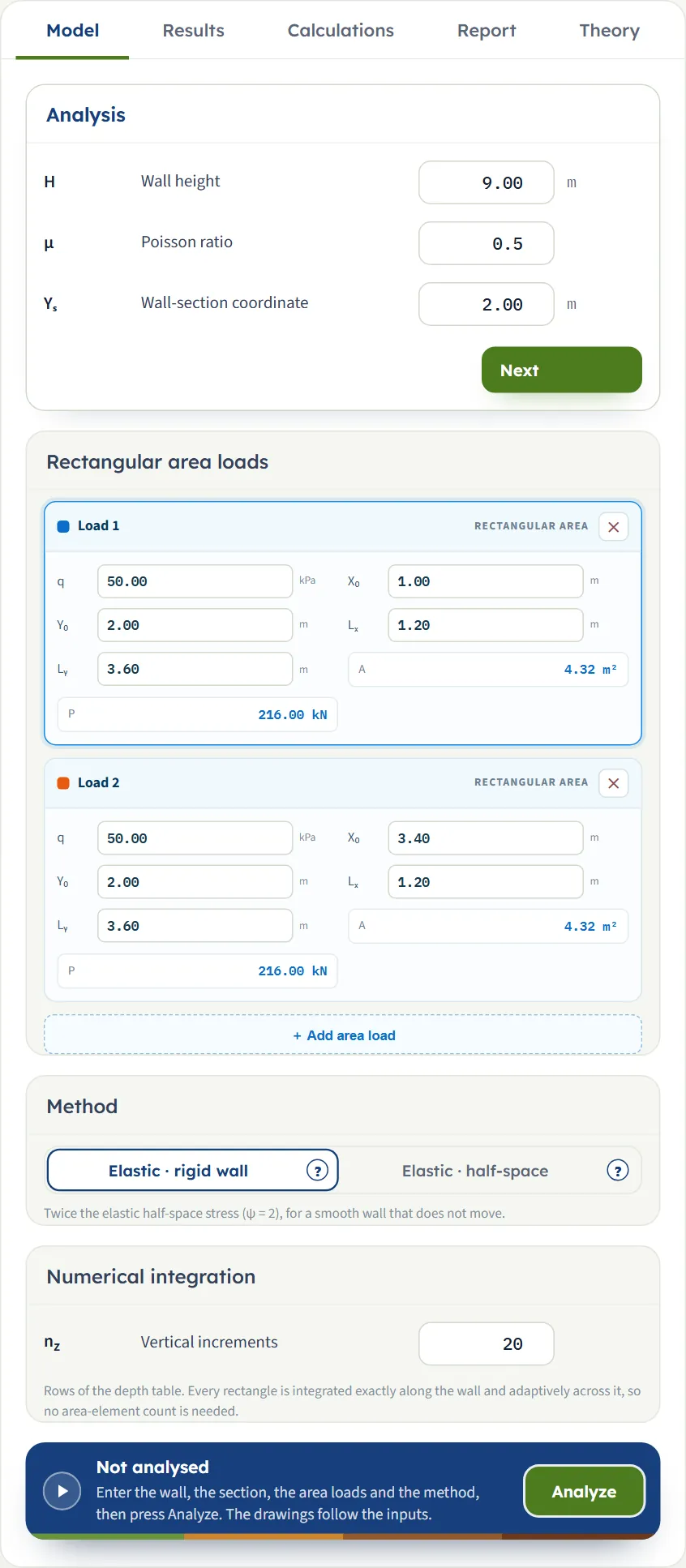
In Analysis, type the wall height H, Poisson’s ratio μ and the section coordinate Ys.
- Describe the loads
In Rectangular area loads, fill in q, X0, Y0, Lx and Ly of Load 1 and Load 2, or drag them on the drawing. Press + Add area load for another rectangle and the cross on a card to remove one.
- Choose the method
In Method, pick Elastic · rigid wall (the default) or Elastic · half-space. The (?) beside each opens a window with a sketch of what it assumes.
- Set the rows of the table
In Numerical integration, leave nz at 20, or change the number of rows of the depth table. From 2 rows upwards the answers do not depend on it.
- Press Analyze
Press Analyze at the foot of the Model tab. The bar reads Analysed, the inputs lock, and the pressure diagram and the resultants appear on the drawing.
- Read the answer
The Results tab gives the peak pressure, the base shear Vx(H), the base moment My(H) and the resultant depth, and the share of each load. The Elevation, Plan and 3D View buttons change the view.
- Take the working and the report
The Calculations tab shows the five steps with your numbers. The Report tab saves a PDF or a Word file.
The screen: three views and the loads you can drag
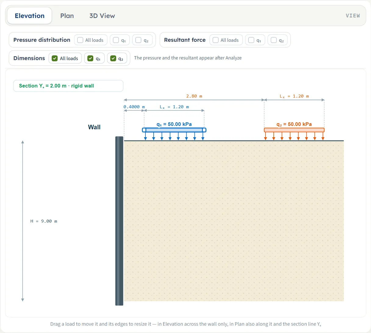
The layout is the one every GeoTerva module shares, described in the workspace guide. In this module the Model tab is one page of four sections, and the drawing has three views, chosen with the buttons above it. Before Analyze a view shows the geometry alone: the wall, the ground, the loads with their values and the dimensions. After Analyze the pressure and the resultants are added.
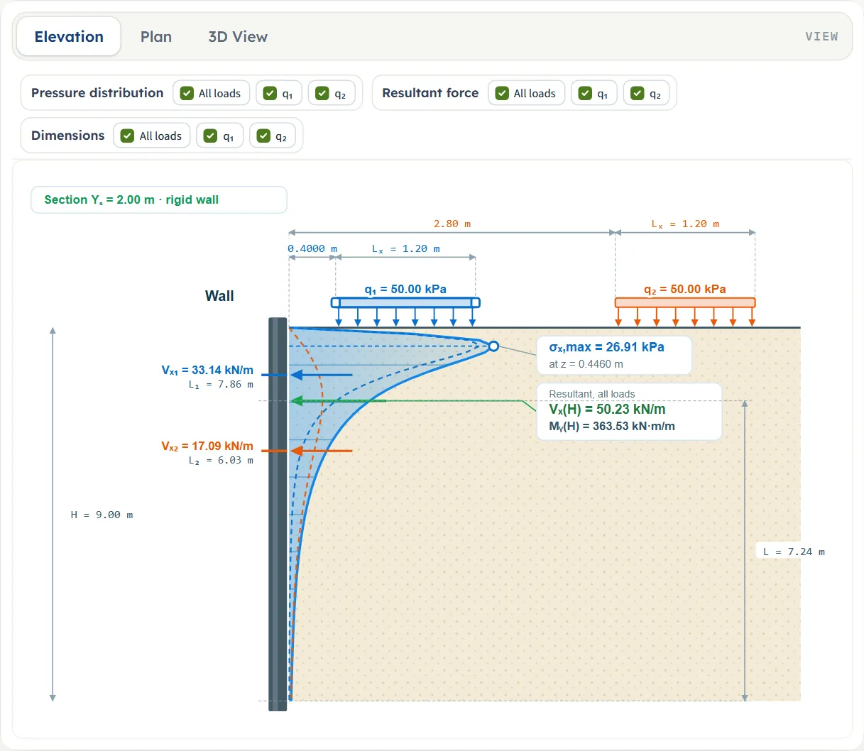
- Elevation is a section through the wall at Ys: the wall, the ground and each load as a bar with arrows and its value. The dimension lines give the distance from the wall to the near edge of each load and its width Lx. After Analyze it adds the pressure diagram on the wall, the peak σx,max with its depth, the resultant of each load alone (Vx and its height L above the base) and the resultant of all the loads with Vx(H), My(H) and its height above the base.
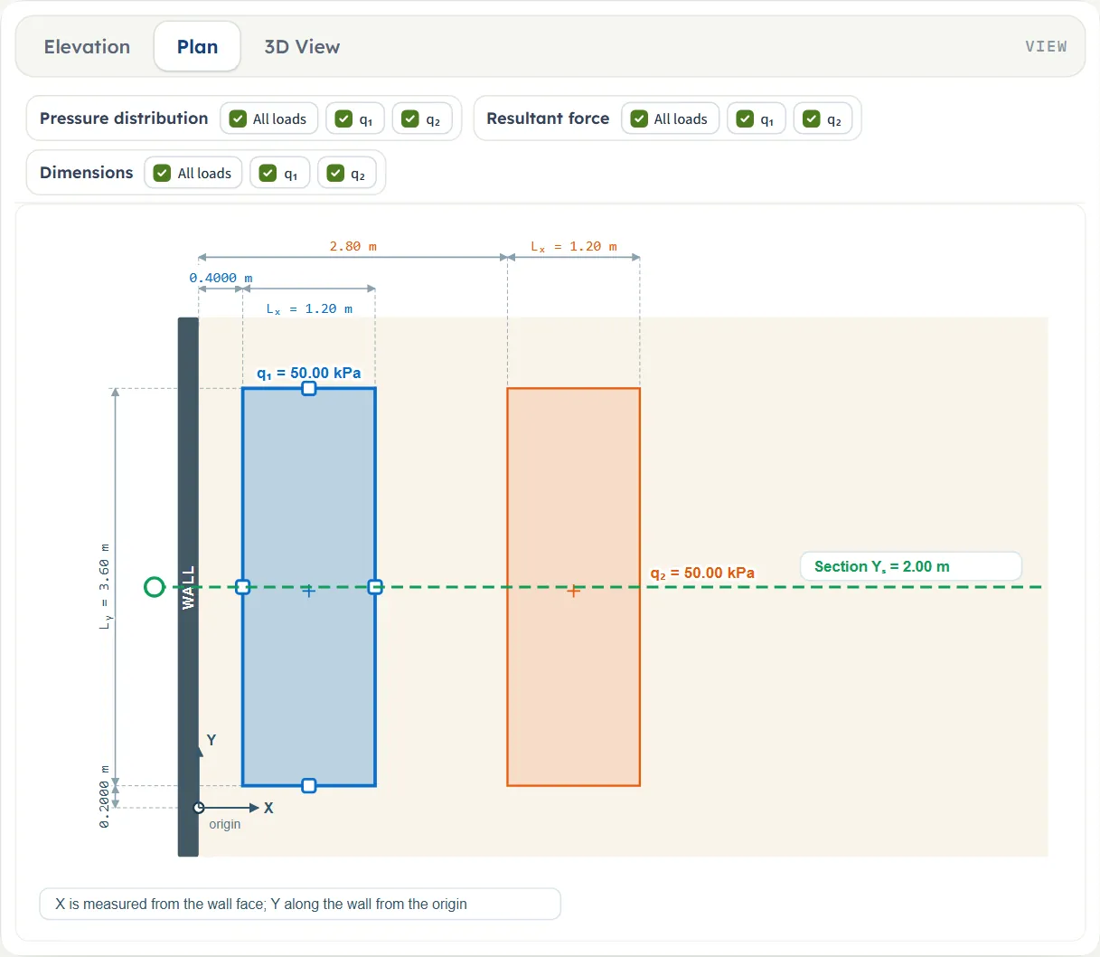
- Plan looks down on the ground. The wall is on the left with the origin and the axes: X is measured from the wall face, Y along the wall from the origin. Each load is a coloured rectangle with its value; the dashed green line is the section Ys. The dimensions give the near edge, Lx, the lower edge and Ly. The plan is the same before and after Analyze.
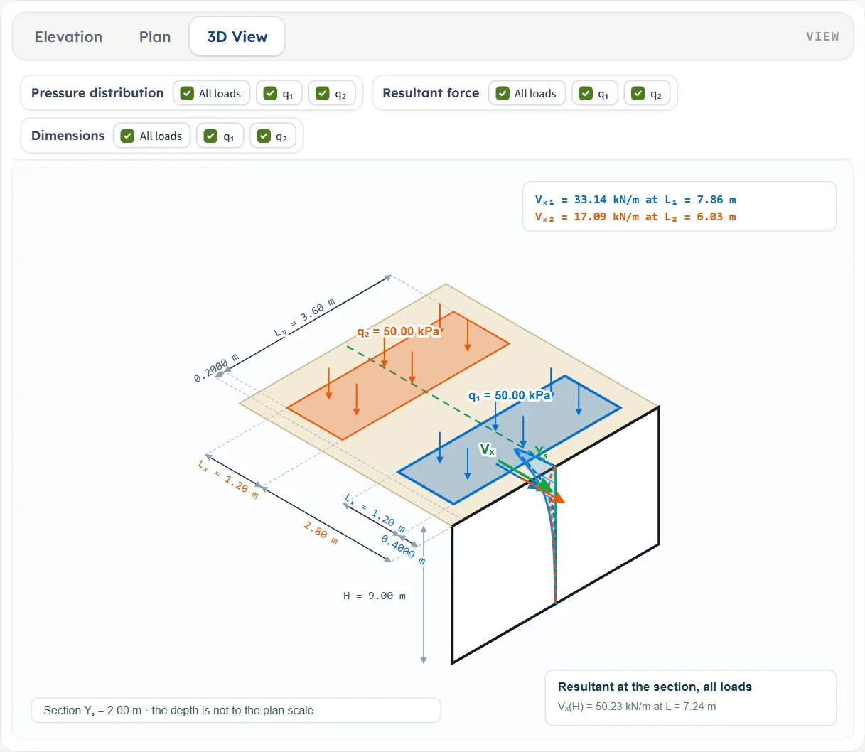
- 3D View shows the wall, the loaded ground and, after Analyze, the pressure on the section, the resultants and the dimensions. A box at the top lists the resultant of each load, and a box at the foot the resultant of all of them.
Choosing and moving a load
Click a load’s card in the Model tab, or the load on the drawing, to select it: its card is outlined, and its handles appear on the drawing. The note under the drawing reads “Drag a load to move it and its edges to resize it — in Elevation across the wall only, in Plan also along it and the section line Yₛ”. Dragging changes the boxes in the Model tab, so the two always agree.
| View | What you drag | What changes |
|---|---|---|
| Elevation | The body of a load | X0: the load moves across the wall, towards or away from it. Y0 does not change. |
| Elevation | The near or far end of a load bar | X0 and Lx: the near or the far edge moves. |
| Plan | The body of a load | X0 and Y0: the load moves in both directions. |
| Plan | A side of a load (the small squares of the selected load) | The near or far edge (X0, Lx), or the lower or upper edge (Y0, Ly). |
| Plan | The section line, by its circle beside the wall or by the dashed line itself | Ys. |
| 3D View | Nothing | The 3D view shows the model; change it in the other views or in the Model tab. |
A dragged edge or position snaps to 0.05 m (0.05 ft in US units). A side cannot be made narrower than 0.05 m, and a load cannot be dragged across the wall face: its near edge stops at the wall. Dragging is available before Analyze; after it the inputs are locked, the note under the drawing is hidden, and Edit inputs unlocks them.
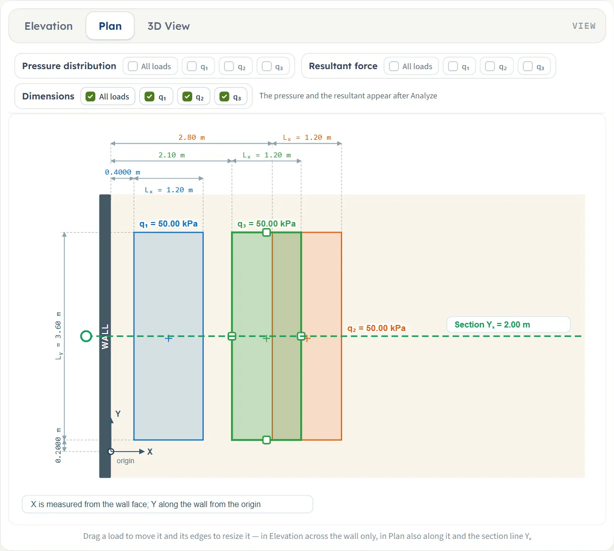
The Show chips
Above the drawing a Show bar controls what is drawn. With one load it has three chips, Pressure distribution, Resultant and Dimensions. With two or more loads it has three groups: Pressure distribution, Resultant force and Dimensions, each with an All loads chip for the sum and one chip for each load (q1, q2, … in the colour of the load). The pressure and the resultant chips are available after Analyze; until then the bar says “The pressure and the resultant appear after Analyze”. The Dimensions chips can be switched at any time.
The pressure chip of a load draws the diagram of that load alone as a dashed curve in its colour, and its resultant chip draws the arrow of that load alone. They are useful to see which load governs. The Resultant chips act on the elevation and the 3D view; the plan has no place for a resultant.
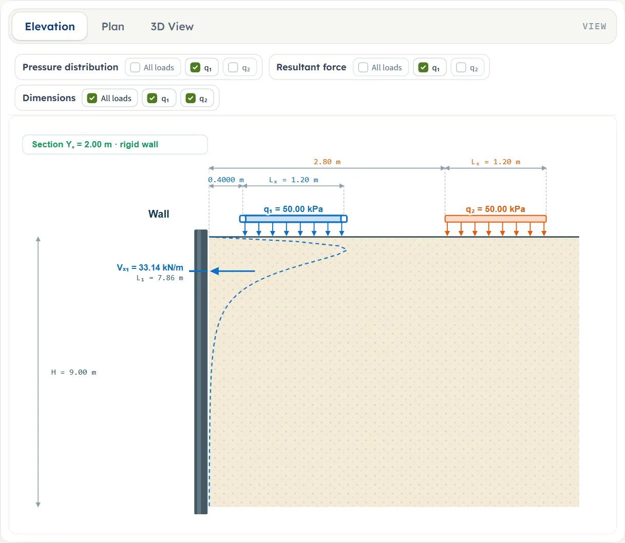
Entering the model, section by section
The Model tab has four sections, always on the page: Analysis, Rectangular area loads, Method and Numerical integration. All four sections stay on the page; Next and Back at the foot of the highlighted section move the highlight to the next or the previous one and scroll to it, and Analyze waits below the last. The tables list every field with its symbol, the unit in each unit system and its default. Where a unit is shown twice or three times, such as m · ft, the units are those of SI · kN, SI · tf and US in turn, and equal ones are merged. Defaults are shown in SI. In SI · tf the load box shows 5.10 t/m²; in US the boxes show 29.53 ft for the wall, 6.56 ft for Ys, 1.04 ksf, 3.28 ft, 6.56 ft, 3.94 ft and 11.81 ft for Load 1.
Analysis
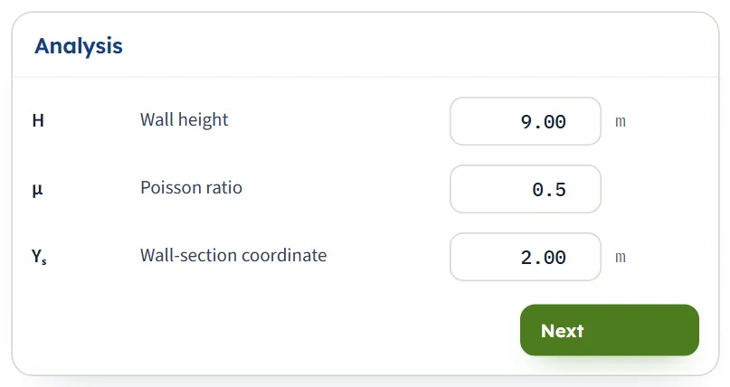
The wall and the section.
| Field | Symbol | Unit | Default | What to enter |
|---|---|---|---|---|
| Wall height | H | m · ft | 9 | The height of the wall over which the pressure is integrated, from the ground surface to the base. It must be greater than zero. |
| Poisson ratio | μ | — | 0.5 | Poisson’s ratio of the soil, from 0 to 0.5. At 0.5 the term (1 − 2μ) of the stress formula vanishes; below 0.5 a small tension appears near the surface. |
| Wall-section coordinate | Ys | m · ft | 2 | The section along the wall at which the pressure is evaluated, measured along the wall from the same origin as Y0. Any number. |
Rectangular area loads
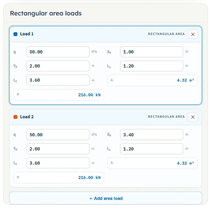
One card for each load, numbered and coloured: the colour is the one the load has in the drawings and in the Show chips. A card has the five fields below (the defaults are those of Load 1; Load 2 differs in X0), and two values the module works out for you and cannot be edited: the area A = LxLy and the load P = qA in kN (tf or kip).
| Field | Symbol | Unit | Default | What to enter |
|---|---|---|---|---|
| q | q | kPa · t/m² · ksf | 50 | The surcharge on the rectangle, as a pressure. Zero or more. |
| X₀ | X0 | m · ft | 1 (Load 1), 3.4 (Load 2) | Distance of the centre of the rectangle from the wall face. At least Lx/2, so that the rectangle lies behind the wall face. |
| Y₀ | Y0 | m · ft | 2 | Position of the centre along the wall, from the same origin as Ys. |
| Lₓ | Lx | m · ft | 1.2 | Side across the wall (perpendicular to the wall face). Greater than zero. |
| Lᵧ | Ly | m · ft | 3.6 | Side along the wall. Greater than zero. |
Adding, removing and selecting loads
- + Add area load adds a rectangle. It starts as a copy of the selected load, with the same q, Y0, Lx and Ly, placed just beyond its far edge: X0 is moved on by Lx plus 0.5 m (0.5 ft in US units). The new load becomes the selected one. If the place is already taken by another load, the two overlap, and the pressures of overlapping loads add (the what-if table shows the effect); type or drag the new load to where you want it.
- The cross (✕) on a card removes that load. It is there when there are two or more loads: one load always remains.
- Up to 20 loads. At 20 the button reads “Up to 20 area loads” and is disabled.
- A load is selected by clicking its card, by typing in one of its boxes, or by clicking it on the drawing. The selected load is outlined on its card and has handles on the drawing.
- A box with a value the module cannot use (a negative q, a side of zero, a load that crosses the wall face) stops the analysis and the message names the load (see Messages).
Method
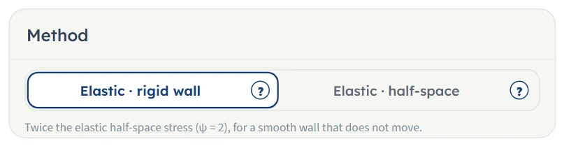
Two buttons, each with a (?). The line under them states the factor of the option chosen. They are described in Choosing the method.
Numerical integration
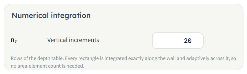
One number, the rows of the depth table of the working. Every rectangle is integrated exactly along the wall and adaptively across it, so no number of area elements is asked for.
| Field | Symbol | Unit | Default | What to enter |
|---|---|---|---|---|
| Vertical increments | nz | — | 20 | The number of rows of the depth table, H/nz apart: a whole number from 1 to 200. From 2 rows upwards it does not change any result (see How each input changes the answer); keep it at 2 or more. |
Choosing the method, μ and the section
The two methods
| Option | Wall factor | What it assumes | Use it when |
|---|---|---|---|
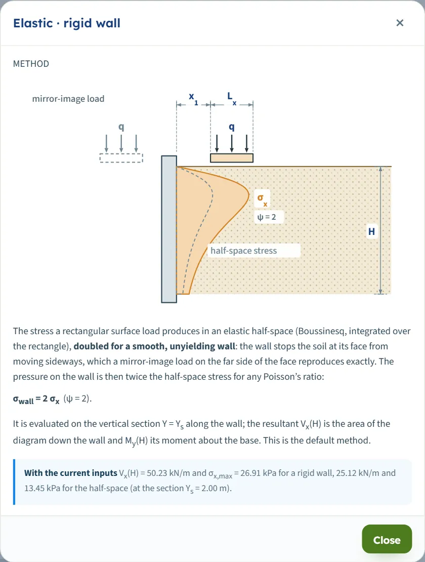
| Elastic · rigid wall (the default) | ψ = 2 | A smooth wall that does not move. Mirroring every load across the wall face cancels the wall-normal displacement and the shear on that plane, so the pressure on the wall is exactly twice the half-space stress, for any Poisson’s ratio. | The wall is a smooth wall that does not move. |
| Elastic · half-space | ψ = 1 | The elastic stress in a half-space, as if the wall were absent. | The wall deflects enough to relieve the soil. |
The second gives half the first everywhere: on the module’s example σx,max is 26.91 kPa for a rigid wall and 13.45 kPa for the half-space, and Vx(H) is 50.23 and 25.12 kN/m. The depth of the peak and the resultant depth are the same. The (?) beside each option opens a window with a sketch of the wall, the load and the pressure for that option, the formula, and a line headed With the current inputs that gives Vx(H) and σx,max for both methods at your inputs.
Reading a window changes nothing in the model.
Poisson’s ratio μ
μ enters the stress formula through the term (1 − 2μ). At the default of 0.5 the term is zero. With μ below 0.5 the pressure is smaller (on the example), and the elastic solution gives a small tension near the surface; the module then shows a caution and keeps the sign in the results (see Messages). On the example, μ = 0.3 gives Vx(H) = 32.72 kN/m, against 50.23 kN/m at 0.5.
The section Ys
The module gives the pressure at one vertical section of the wall, at Y = Ys. The loads need not cross it: a load that does not reach the section still contributes, less the farther it is, and the Results tab marks it “off the section”. To find the most loaded part of the wall, run the module at several sections: on the example, the section through the centre of the loads gives Vx(H) = 50.23 kN/m, and a section 0.2 m beyond the end of the loads gives 26.36 kN/m.
The rows nz
nz sets how many rows the table of the wall integration has. The shear force and the moment are integrated between the rows, not summed from them. From 2 rows upwards, nz does not change any result: nz = 5 and nz = 100 give the same answers as 20. With 1 row the shear, the moment and the resultant depth are the same, but the peak pressure is read from the two table rows only, so keep nz at 2 or more (the default is 20).
Analyze and read the results
Press Analyze. The bar changes to Analysed — the lateral pressure calculated and says “The inputs are locked. Edit inputs clears the results; the unit system can still be changed.” The Results tab shows eight cards and a list of the loads, and the drawing now carries the pressure and the resultants.
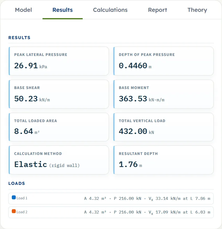
| Card | Symbol | What it is | The example |
|---|---|---|---|
| Peak lateral pressure | σx,max | The largest ordinate of the pressure diagram on the wall at the section. | 26.91 kPa |
| Depth of peak pressure | z | The depth below the ground at which the peak occurs. | 0.4460 m |
| Base shear | Vx(H) | The resultant of the pressure on the wall, per unit length of wall: the shear force at the base. | 50.23 kN/m |
| Base moment | My(H) | The moment of the pressure about the base, per unit length of wall. | 363.53 kN·m/m |
| Total loaded area | The sum of the areas LxLy of all the loads. | 8.64 m² | |
| Total vertical load | The sum of qLxLy: the load on the ground, not the load on the wall. | 432.00 kN | |
| Calculation method | Elastic, with the wall in brackets: (rigid wall) or (half-space). | Elastic (rigid wall) | |
| Resultant depth | zR | The depth below the ground at which Vx(H) acts. Its height above the base is H − zR. | 1.76 m |
The Loads list
Below the cards each load has a line with its colour, its area A and its load P. With two or more loads the line also gives the shear force Vx of that load alone and the height L of its resultant above the base, the same numbers as the arrows on the drawing: on the example Load 1 gives 33.14 kN/m at 7.86 m and Load 2 gives 17.09 kN/m at 6.03 m, and the two add up to 50.23 kN/m. A load whose length along the wall does not include the section is marked “off the section”.
Using the numbers
- Vx(H) and My(H) are per unit length of wall at the section. Add the pressure diagram, or Vx(H) acting at the height H − zR above the base, to the earth-pressure and water-pressure diagrams of the wall calculation.
- The resultant of the sum is drawn on the elevation with its height above the base (L = 7.24 m on the example, which is H − zR = 9 − 1.76 to the rounding of the figures).
- Changing the unit system after Analyze re-states the cards, the drawing and the report without a new run. Edit inputs unlocks the model and clears the results.
The Calculations tab and the report
The Calculations tab writes out the working in five numbered steps, each with its equations, a short note and the numbers:
- Wall, section and method — the method with its factor ψ, H, μ and Ys, and a table of the loads: q, X0, Y0, Lx, Ly, A and P.
- Rectangles relative to the section — x1 = X0 − Lx/2, x2 = X0 + Lx/2, y1 = Y0 − Ly/2 − Ys and y2 = Y0 + Ly/2 − Ys for each load, with their values.
- Point-load stress (Boussinesq) — the horizontal stress σx perpendicular to the wall under a point load.
- Integration over each rectangle — the integral along the wall and across it; at the depth of the peak the stress of each load and their sum σx,max; then the table of the wall integration, every H/nz: z, σx, Vx and My.
- Shear force and bending moment — Vx(H), My(H) and the resultant depth zR.
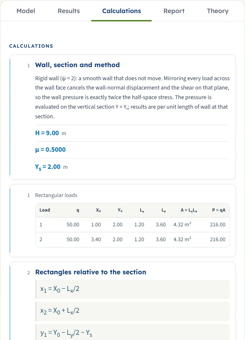
Before Analyze the tab says “Press Analyze on the Model tab to calculate the lateral pressure.” Cautions and notes of the run appear at the end of the working.
The report
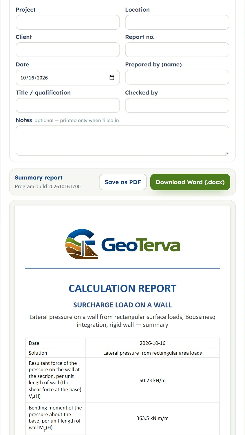
In the Report tab fill in the cover: Project, Location, Client, Report no., Date, Prepared by (name), Title / qualification, Checked by and optional Notes. The details are kept in this browser. After Analyze, Save as PDF and Download Word (.docx) are available; before it they are greyed out, and the tab says “Press Analyze on the Model tab to calculate the lateral pressure.”
The report has six parts: 1 Introduction and scope, 2 Input data, 3 Calculation (3.1 to 3.5, one for each step), 4 Results, 5 Summary and 6 References. It carries the elevation, the plan and the 3D drawing, and states the units with the conversion constants. When the run has a caution or a note, an Assumptions and notes part is added after Results, and the parts after it move down by one.
The Theory tab has six sections: Area loads on a wall, Stress from a point load, Integrating a rectangle, Shear force and bending moment, a worked example and References.
Worked example: the module’s own example
The module opens on this example, so you can follow the numbers on your own screen.
| Section | Input | Value |
|---|---|---|
| Analysis | Wall height, Poisson’s ratio, section | H = 9 m, μ = 0.5, Ys = 2 m |
| Rectangular area loads | Load 1 | q = 50 kPa, X0 = 1 m, Y0 = 2 m, Lx = 1.2 m, Ly = 3.6 m |
| Rectangular area loads | Load 2 | The same, with X0 = 3.4 m |
| Method | Method | Elastic · rigid wall (ψ = 2) |
| Numerical integration | Rows | nz = 20 |
Step 1: the loads and their position
Each rectangle has the area A = 1.2 × 3.6 = 4.32 m² and the load P = 50 × 4.32 = 216.00 kN; together 8.64 m² and 432.00 kN. Relative to the wall and the section: x1 = 1 − 0.6 = 0.4 m and x2 = 1 + 0.6 = 1.6 m for Load 1, 2.8 to 4.0 m for Load 2; for both, y1 = 2 − 1.8 − 2 = −1.8 m and y2 = 2 + 1.8 − 2 = 1.8 m, so the section runs through the middle of both.
Step 2: the pressure on the wall
The stress under a point load is integrated over each rectangle and doubled for the rigid wall. The sum has its peak at the depth z = 0.4460 m: Load 1 gives 24.98 kPa there, Load 2 gives 1.93 kPa, and σx,max = 24.98 + 1.93 = 26.91 kPa. The pressure then falls quickly with depth. The table of the wall integration, as the Calculations tab gives it:
| z (m) | σx (kPa) | Vx (kN/m) | My (kN·m/m) |
|---|---|---|---|
| 0.00 | 0.00 | 0.00 | 0.00 |
| 0.4500 | 26.91 | 8.45 | 1.45 |
| 0.9000 | 20.89 | 19.44 | 7.84 |
| 1.80 | 10.31 | 32.80 | 32.06 |
| 3.60 | 3.46 | 43.85 | 102.82 |
| 5.40 | 1.35 | 47.85 | 185.91 |
| 9.00 | 0.2848 | 50.23 | 363.53 |
Step 3: the resultant and the moment
The shear force grows with depth and reaches Vx(H) = 50.23 kN/m at the base: 33.14 from Load 1 and 17.09 from Load 2. The moment about the base is My(H) = 363.53 kN·m/m, and the resultant acts at zR = 1.76 m below the ground, that is 7.24 m above the base, which the elevation shows as L. As a check, Vx(H) (H − zR) = 50.23 × (9 − 1.76) = 363.7 kN·m/m, equal to My(H) to the rounding of zR.
The same wall on the half-space
Choose Elastic · half-space (after Edit inputs) and analyze again: σx,max = 13.45 kPa, Vx(H) = 25.12 kN/m and My(H) = 181.77 kN·m/m, exactly half of the rigid-wall values, at the same depths 0.4460 m and 1.76 m.
How each input changes the answer
Each row changes one thing in the example and runs the module again. The numbers are the ones the module gives, so you can reproduce any row.
| Change | σx,max (kPa) | Vx(H) (kN/m) | My(H) (kN·m/m) | zR (m) |
|---|---|---|---|---|
| The default example | 26.91 | 50.23 | 363.53 | 1.76 |
| Half-space method | 13.45 | 25.12 | 181.77 | 1.76 |
| q = 100 kPa on both loads | 53.81 | 100.46 | 727.07 | 1.76 |
| H = 6 m | 26.91 | 48.55 | 214.84 | 1.58 |
| H = 12 m | 26.91 | 50.76 | 515.15 | 1.85 |
| μ = 0.3 | 20.19 | 32.72 | 244.28 | 1.53 |
| Ys = 0 m | 10.26 | 26.36 | 178.85 | 2.21 |
| Ys = 4 m | 10.26 | 26.36 | 178.85 | 2.21 |
| Ys = 8 m | 0.4061 | 2.44 | 11.53 | 4.27 |
| Load 2 removed | 25.03 | 33.14 | 260.49 | 1.14 |
| Load 2 at X0 = 6.4 m | 25.35 | 41.45 | 299.42 | 1.78 |
| Load 1 at X0 = 0.6 m | 50.00 | 52.86 | 399.02 | 1.45 |
| A third load at X0 = 4.6 m | 27.77 | 62.82 | 431.30 | 2.13 |
| A third load added and left where it starts | 30.58 | 70.95 | 497.90 | 1.98 |
| Ly = 10 m on both loads | 28.49 | 66.51 | 455.90 | 2.15 |
| nz = 5 | 26.91 | 50.23 | 363.53 | 1.76 |
| nz = 100 | 26.91 | 50.23 | 363.53 | 1.76 |
What each row shows. The depth of the peak is given where it differs from the example’s 0.4460 m.
- Half-space method. Every value is half of the rigid-wall value; the depths are the same.
- q = 100 kPa on both loads. Doubling q doubles the pressure, the shear and the moment; the depths do not change.
- H = 6 m. The peak is unchanged; the pressure below 6 m is lost, so the moment drops most.
- H = 12 m. A little more shear and moment: the pressure is small at depth.
- μ = 0.3. Lower pressure, and a tension near the surface: a caution is raised (the peak is at 0.4733 m).
- Ys = 0 m. The section is 0.2 m beyond the lower end of the loads (the peak is at 0.5759 m).
- Ys = 4 m. The same, 0.2 m beyond the upper end: the loads are symmetric about Y = 2 m (the peak is at 0.5759 m).
- Ys = 8 m. Far from the loads: small pressure, and the peak is deep (the peak is at 3.09 m).
- Load 2 removed. Load 1 alone: the 33.14 kN/m of its line in the Loads list (the peak is at 0.4189 m).
- Load 2 at X0 = 6.4 m. A farther load contributes less (the peak is at 0.4236 m).
- Load 1 at X0 = 0.6 m. Its near edge is at the wall face: the peak is at the surface and the Calculations tab notes it (the peak is at 0.00 m).
- A third load at X0 = 4.6 m. Same size, behind the other two (4.0 to 5.2 m): a smaller addition (the peak is at 0.4599 m).
- A third load added and left where it starts. It starts at X0 = 2.7 m and overlaps Load 2, so it adds much more (the peak is at 0.5019 m).
- Ly = 10 m on both loads. More load along the wall: more pressure at the section (the peak is at 0.4706 m).
- nz = 5. No change.
- nz = 100. No change.
The pattern: the pressure is linear in q and adds up load by load, it falls quickly with distance from the wall and from the section, and the method only scales it by a factor of two.
Messages: stops, cautions and notes
The module checks the numbers it needs. When one cannot be used it stops, and nothing is calculated; when a result needs care it raises a caution; and it adds a note where it assumed something.
Stops
- A red message appears in the Model tab above the Analyze bar, and the bar turns brown and reads Cannot be analysed, followed by the message.
- If you press Analyze, a window titled Cannot be analysed gives the message and says “Nothing was calculated. Change the inputs marked in red, then press Analyze again.”
- The Results tab says “Not calculated — see the Model tab.”, and the drawings say “Not calculated — correct the highlighted input in the Model tab”.

| Kind | When | Message and what to do |
|---|---|---|
| Stop | The wall height is zero, negative or empty | “The wall height H must be greater than zero.” Enter a height above zero. |
| Stop | μ is outside 0 to 0.5, or empty | “Poisson's ratio μ must lie between 0 and 0.5.” Enter a value in that range. |
| Stop | Ys is empty | “The section coordinate Yₛ must be a number.” Enter the section. |
| Stop | nz is not a whole number from 1 to 200 | “The vertical increments nz must be a whole number from 1 to 200.” Enter a whole number in that range. |
| Stop | A load whose near edge is in front of the wall face (X0 < Lx/2) | “Load 1 crosses the wall face: X₀ must be at least Lₓ/2.” (the number is that of the load) Increase X0 or reduce Lx. |
| Stop | A load with a negative or empty q, or a side that is zero, negative or empty | “Load 2: q must be zero or more and Lₓ, Lᵧ greater than zero.” (the number is that of the load) Correct the load named. |
Every stop continues with the same two sentences: “Every rectangle must lie behind the wall face (X ≥ 0) with positive plan dimensions, on a wall of positive height. Correct the highlighted value in the Model tab.” When more than one value is wrong, the messages are joined in one stop, separated by semicolons, for example “Load 1 crosses the wall face: X₀ must be at least Lₓ/2; Load 2: q must be zero or more and Lₓ, Lᵧ greater than zero.”
Caution and note
| Kind | When | Message and what to do |
|---|---|---|
| Caution | Some ordinates of the pressure are negative, which happens when μ is below 0.5 | “Some ordinates are negative (tension). With μ below 0.5 the elastic solution gives a small tension near the surface, and soil cannot pull on a wall. The sign is kept in the results; ignore the negative part if it is not wanted.” It appears in the Model tab, at the end of the Calculations tab and in the report, in a part called Assumptions and notes. |
| Note | A load starts at the wall face (X0 = Lx/2) | “A load starts at the wall face. The stress under a load edge on the wall is singular at the surface; the integrals stay finite and are evaluated adaptively.” It appears in the Calculations tab and in the report. |
With μ = 0.3 the first row of the table of the wall integration is σx = −8.36 kPa at the ground surface for the example. With μ = 0 the example gives Vx(H) = 6.45 kN/m and a resultant depth of −1.14 m: the tension near the surface then outweighs the pressure there, and the diagram is the better guide than the single number.
Good practice and common mistakes
- Measure X0 to the centre. X0 is the distance from the wall face to the centre of the rectangle, not to its near edge. The near edge is X0 − Lx/2, and the dimension lines of the drawing show it.
- Use one origin along the wall. Y0 of every load and Ys are measured from the same origin. A section that does not lie within the length of a load is not wrong, but it gives a smaller pressure.
- Look for the governing section. The module gives the pressure at one section. Run it at the section through the middle of the heaviest load and at the others that matter, and design for the largest.
- Choose the method from the wall. Rigid wall for a smooth wall that does not move, half-space for a wall that deflects enough to relieve the soil; the rigid-wall values are twice the half-space ones.
- Watch overlapping loads. A load added to the list starts beside the selected one and can overlap another. Overlapping rectangles add their pressures, so move or retype it.
- Keep μ at 0.5 unless you have a reason. Lower values reduce the pressure and bring a tension near the surface; the module keeps the sign.
- Use the Show chips to see which load governs. The dashed curve and the arrow of each load alone are on the drawing.
- Enter q as a pressure, load per unit area, not as a force. The module shows the load P = qA beside each card as a check.
- Read the results per unit length. Vx(H) is in kN/m of wall at the section, and My(H) in kN·m/m.
- Add the result to the other pressures. The result is the surcharge component only; the wall calculation combines it with the earth pressure and the water pressure.
- Note your values. The module opens on its example every time and does not keep what you typed; the report is the record of an analysis.
- Check the units after switching the system: type values in the units shown beside the boxes.
Frequently asked questions
How do I calculate the lateral pressure on a wall from a rectangular surface load?
The horizontal stress under a point load (Boussinesq) is integrated over the rectangle and the stresses of all the rectangles add; for a wall that does not move the result is doubled. In GeoTerva’s Area loads module you enter the wall height, the section along the wall and, for each load, the pressure, the position of its centre and its two sides, press Analyze, and read the pressure diagram, the resultant Vx(H), its depth and the moment My(H). For the module’s example, Vx(H) = 50.23 kN/m and σx,max = 26.91 kPa.
What is the difference between the rigid-wall and the half-space method?
The rigid-wall method (ψ = 2) is for a smooth wall that does not move: a mirror-image load across the wall face cancels the wall-normal displacement, so the pressure on the wall is twice the half-space stress. The half-space method (ψ = 1) takes the elastic stress as if the wall were absent, for a wall that deflects enough to relieve the soil. The second gives exactly half the first everywhere.
What is the section Ys?
The vertical line along the wall at which the pressure is worked out. The module gives the pressure diagram, the resultant and the moment per unit length of wall at that section. Loads that do not reach the section still contribute, less the farther away they are. Run the module at the sections that matter and design for the largest.
How are X0, Y0, Lx and Ly measured?
X0 is the distance from the wall face to the centre of the rectangle and Lx its side across the wall, so the near edge is at X0 − Lx/2 and must not be in front of the wall. Y0 is the position of the centre along the wall and Ly the side along it. Y0 and the section Ys are measured from the same origin, which you place where you like.
How many loads can I enter, and how do I move one?
Up to 20. Press + Add area load for another, and the cross on a card to remove one. To move a load, type new values or drag it on the drawing: in Plan the body moves it in both directions, a side resizes it, and the section line has its own handle; in Elevation a load moves across the wall only. The 3D view is not draggable.
Do overlapping loads add?
Yes. The pressures of the rectangles add, so two rectangles on the same ground are counted twice. A load added with Add area load starts as a copy of the selected one, just beyond its far edge, and can overlap another load: move it or retype it.
Why does a lower Poisson’s ratio give a caution?
The stress formula has a term (1 − 2μ) that is zero at μ = 0.5. Below 0.5 the elastic solution gives a small tension near the surface, and soil cannot pull on a wall. The module keeps the sign in the results and says so; ignore the negative part if it is not wanted.
What values does the module accept?
The wall height greater than zero, μ from 0 to 0.5, a number for Ys, nz a whole number from 1 to 200, and for each load q of zero or more, positive sides Lx and Ly, and X0 of at least Lx/2. Anything else stops the analysis with a message, which names the load.
Does the number of rows nz change the answer?
Not from 2 rows upwards. It sets the rows of the table of the wall integration, and the shear force and the moment are integrated between the rows, so the answers do not depend on it. With 1 row the shear, the moment and the resultant depth are the same, but the peak pressure is read from the two table rows only, so keep nz at 2 or more (the default is 20).
Does the result include the earth pressure of the soil and the water pressure?
No. The result is the surcharge component only. You add it to the earth-pressure and water-pressure diagrams in the wall calculation.
Which units does it use, and what are the units of the answer?
SI · kN, SI · tf or US, switchable in the header at any time, even after Analyze. Pressures are in kPa, t/m² or ksf, the resultant per unit length in kN/m, tf/m or kip/ft, the moment per unit length in kN·m/m, tf·m/m or kip·ft/ft, and lengths in m or ft.
Does the module remember my inputs?
No. It opens on its example (a 9 m wall and two loads of 50 kPa) each time the page is opened. The unit system and the report cover details you type are kept in the browser. The report is the record of an analysis.