

What the module calculates
Point load gives the extra horizontal pressure that a concentrated load on the ground behind a vertical wall puts on the wall. For a wall of height H, a load Qp on the ground surface and its horizontal distance x from the wall, it returns the pressure diagram down the wall, on the load’s own section, and two numbers that describe it:
PH is the resultant of the pressure, a force per metre of wall, and L is the height of the resultant above the base of the wall: the area and the centroid of the pressure diagram. The module also gives the peak pressure σH,max and the depth where it occurs. Each result is drawn on the wall in elevation, in plan and in 3D.
What you can describe
- A wall of height H, and one to three point loads, each with its own distance x and its own load Qp. All the loads stand on one line perpendicular to the wall, and their pressures add.
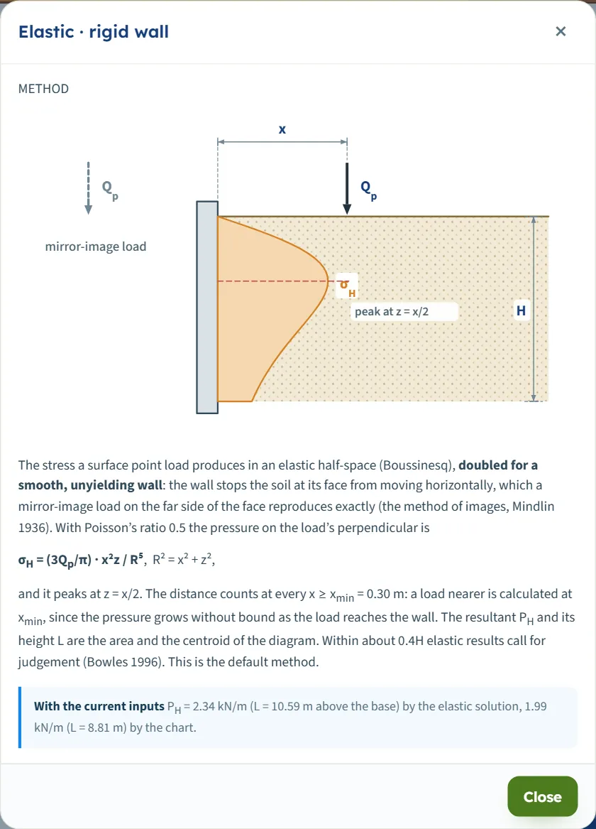
- Two methods: the elastic solution for a rigid wall (the default; twice the Boussinesq stress, Mindlin 1936) and the Terzaghi–NAVFAC chart (Terzaghi 1954).
- Three unit systems, switched in the header: SI · kN, SI · tf and US.
No soil parameter is entered: the pressure follows from the geometry and the load.
What belongs to other modules
- The module gives the pressure that the load adds. The earth pressure, the water pressure and the other actions of a complete wall analysis are separate; the result here is the surcharge component that is combined with them.
- A load spread over a line, a strip, a triangle, a ramp or a rectangle, and a uniform surcharge over the whole surface, have their own modules: Strip load, Line load, Triangular load, Uniform load, Area loads and Ramp load.
- A load that stands on the wall itself or almost against it is better taken as an area load or as a load on the wall; the module says so when a load is that close (see Messages).
Before you start: what you need
Have these ready from your layout drawings and your loading:
| What | Where it comes from | Notes |
|---|---|---|
| Wall height H | Your design | The height of the wall over which the pressure is added up. It must be greater than zero. |
| Point load Qp | Your loading | A concentrated load acting on the ground surface: a wheel, a crane outrigger, a column on a pad, a stack. One value of force for each load. |
| Distance x | Your layout | The horizontal distance from the face of the wall to the load, measured perpendicular to the wall. Zero or more. |
| How many loads | Your layout | Up to three, all on one line perpendicular to the wall. For loads side by side along the wall, work each position in turn: the module gives the pressure on the section through the loads. |
| The method | Your design basis | The elastic solution for a rigid wall (default) or the Terzaghi–NAVFAC chart. Choosing the method compares them. |
Quick start in seven steps
- Open the module and choose the units
Open Point load from the Surcharge Loads family. Pick SI · kN, SI · tf or US in the header; you can change it at any time.
- Enter the wall height
In Geometry, enter the wall height H.
- Choose the method
In Method, pick Elastic · rigid wall (the default) or Terzaghi–NAVFAC chart. The (?) beside each opens a window with a sketch and the equation.
- Describe the load
In Point loads, enter the distance x from the wall and the load Qp. Press + Add point load for a second and a third load, up to three. Or drag the load in the drawing.
- Check the drawing
The drawing follows the inputs: the wall, the load or loads and their distances in Elevation, Plan and 3D View.
- Press Analyze
Press Analyze. The bar turns green, the inputs lock, and the pressure diagram and the resultant appear on the drawings.
- Read the answer
The Results tab gives the resultant force, its depth, the peak pressure and where it occurs; Calculations shows every step; Report saves a PDF or a Word file.
The screen: three views and dragging the load
The layout is the one every GeoTerva module shares, described in the workspace guide. The drawing on the left has three views, chosen with the buttons above it; the Model, Results, Calculations, Report and Theory tabs are on the right.
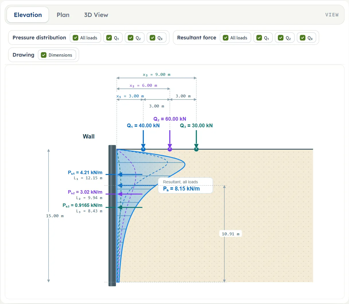
- Elevation is a section through the wall and the load: the wall on the left, the ground to the right, the load as an arrow on the ground surface with its distance x, and the wall height H. After Analyze it adds the pressure diagram on the face of the wall, and the resultant PH as an arrow at its height L above the base.
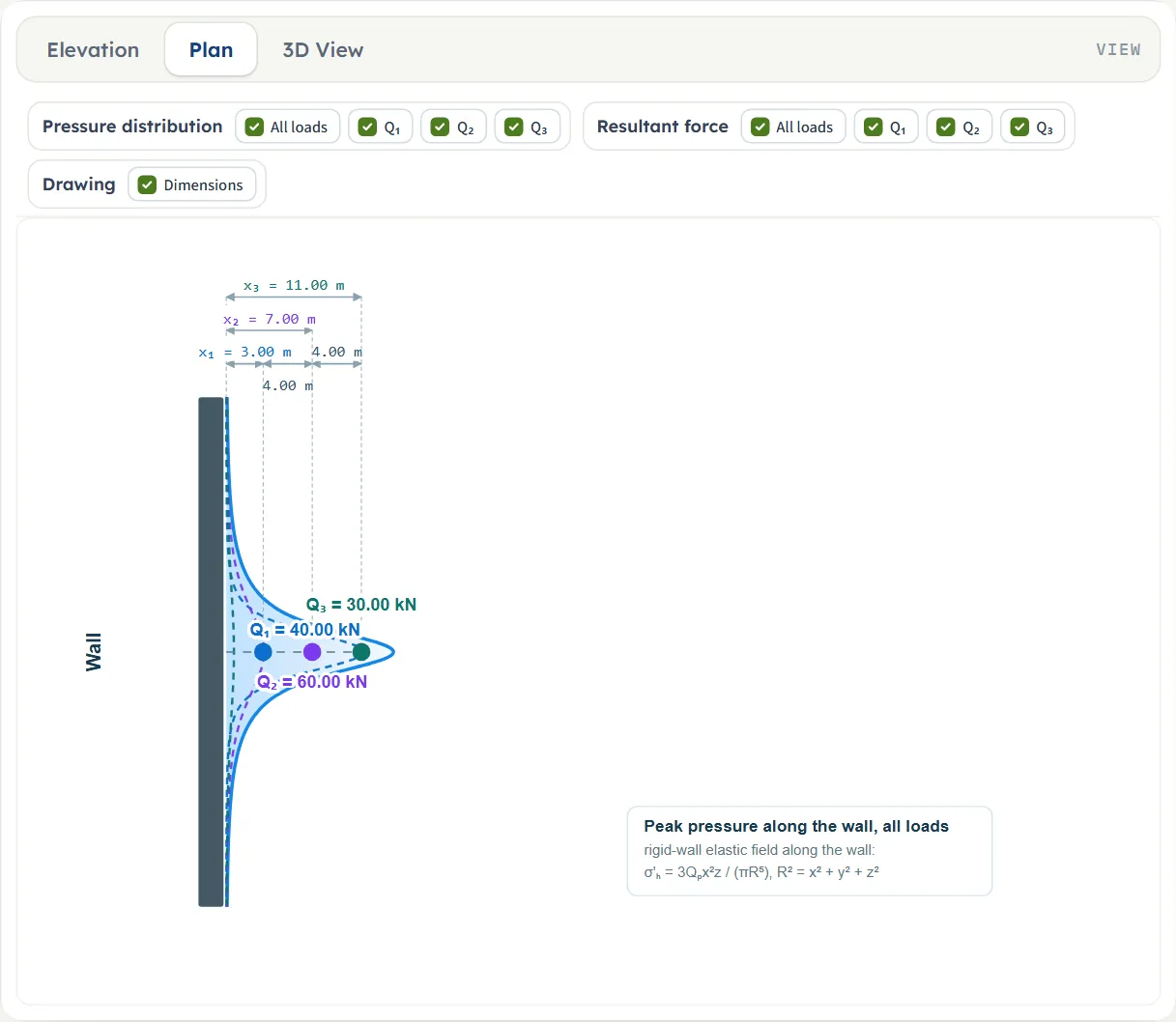
- Plan looks down on the wall and the load. After Analyze it draws how the peak pressure falls away along the wall on either side of the load.
- 3D View shows the wall, the ground and the load in one picture, with the pressure on the wall face, the resultant arrow and a box with PH and L.
Before Analyze the drawings show the geometry alone, and the chips Pressure distribution and Resultant are greyed out, with the note “The pressure and the resultant appear after Analyze”. The chip Dimensions is always available: it switches the dimension lines, their labels and the extension lines on and off.
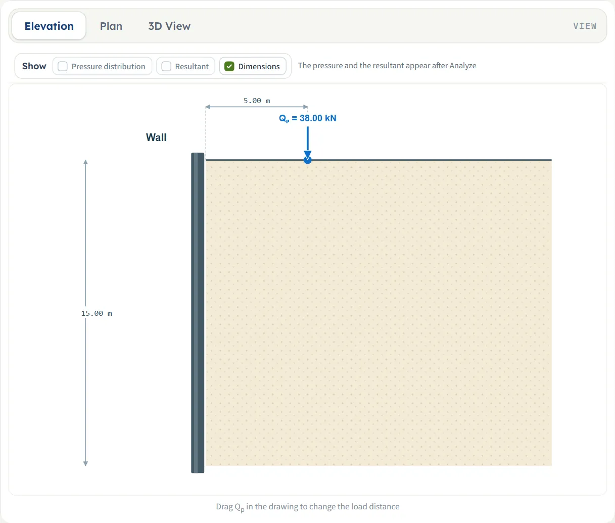
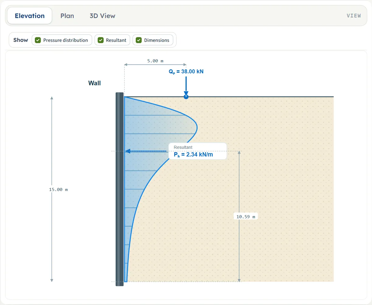
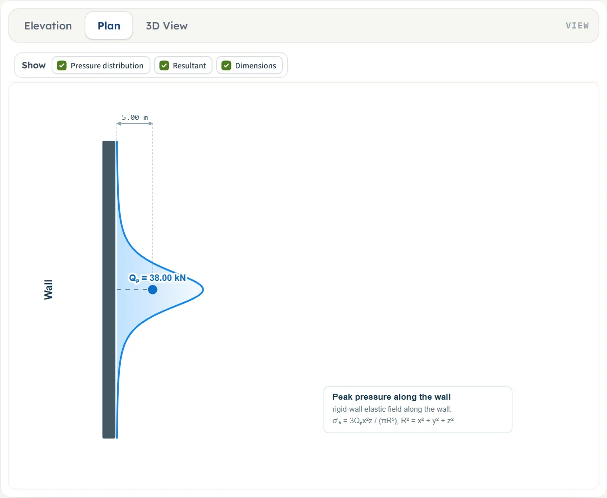
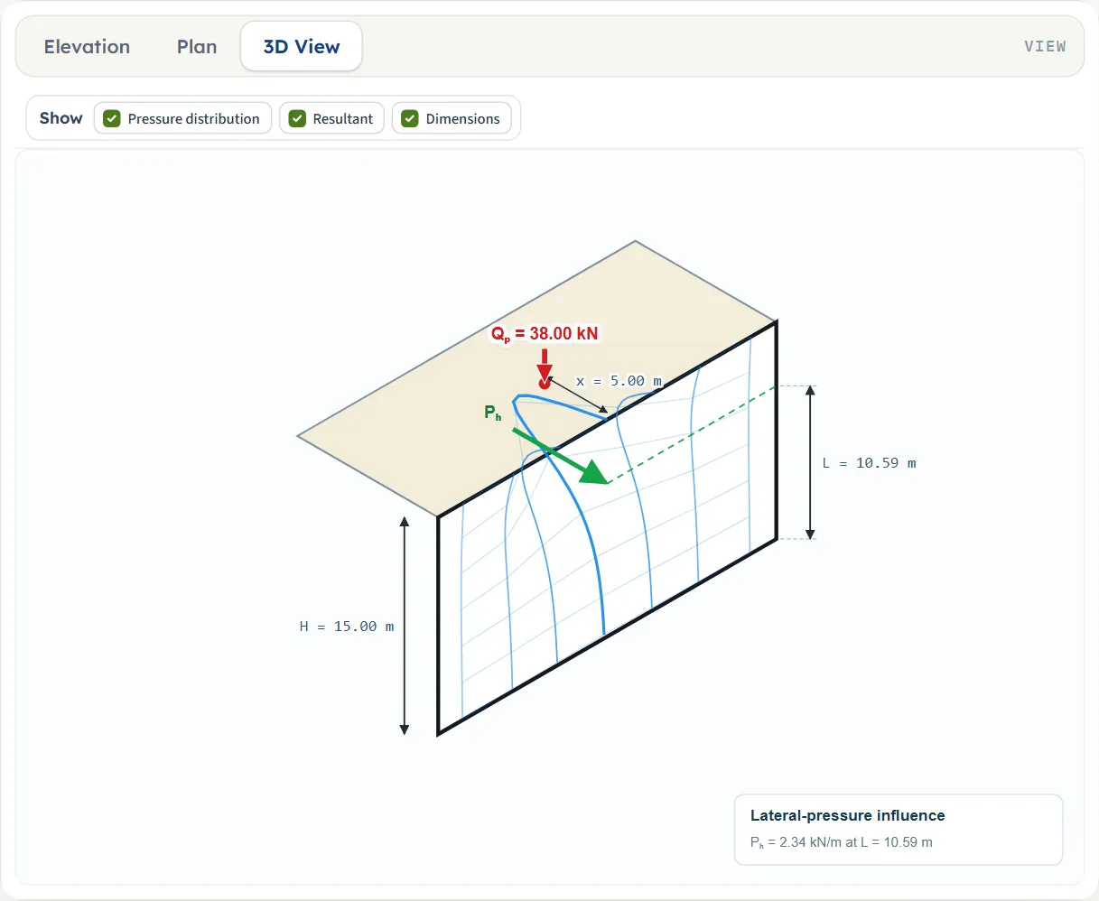
Show chips
After Analyze, Pressure distribution and Resultant switch the pressure diagram and the resultant arrow on and off in the drawings (the resultant is shown in Elevation and in 3D View). With several loads the chips become three groups: the pressure distribution and the resultant force, each with All loads and one chip for every load, and Drawing with Dimensions. The chip of a load carries its colour, the same colour as the load in the drawing and in the Model tab.
Dragging the load
Before Analyze, drag the load in any of the three views to change its distance x: press on the dot at the foot of the arrow and move it along the ground. The box in the Point loads section follows while you drag. The distance snaps to 0.05 of the length unit shown (0.05 m or 0.05 ft) and cannot go below 0 or past the far edge of the drawing in that view. The drawing keeps its scale while you drag and refits when you let go. With several loads each load has its own handle, and the one nearest the pointer is picked up. Dragging changes x only; Qp and H are typed.
The hint “Drag Qp in the drawing to change the load distance” shows below the drawing while the inputs are open. After Analyze the inputs are locked and the load cannot be dragged: press Edit inputs first.
Entering the model, section by section
The Model tab has three sections: Geometry, Method and Point loads. Each opens when you click its title, and Next and Back at the foot walk you through them. Where a unit is shown twice or three times, such as m · ft, the units are those of SI · kN, SI · tf and US in turn, and equal ones are merged. The defaults are shown in SI; in another unit system the boxes show the converted values.
Geometry
The wall height is the only geometry besides the position of the loads.
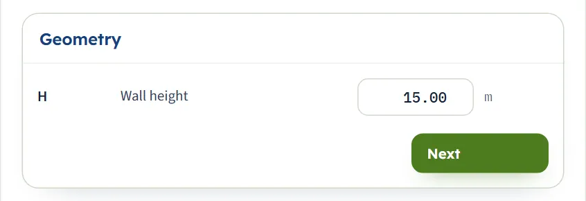
| Field | Symbol | Unit | Default | What to enter |
|---|---|---|---|---|
| Wall height | H | m · ft | 15.00 | The height of the wall over which the pressure is added up. It must be greater than zero. |
Method
Two buttons choose the method; the note under them says what the chosen method does. The (?) beside a method opens a window with a sketch, the equation and a line With the current inputs that gives PH and L by both methods for your values, so you can compare without changing the choice.
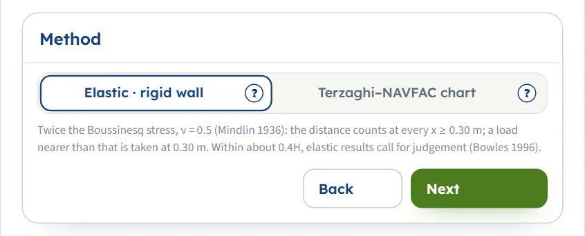
| Choice | Options | Default |
|---|---|---|
| Calculation method | Elastic · rigid wall Terzaghi–NAVFAC chart | Elastic · rigid wall |
Point loads
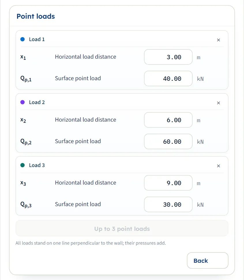
Every load has a card with a colour dot, a cross to remove it, and two boxes. With one load the symbols are x and Qp; with several they are x1, Qp,1 , x2, Qp,2 and so on, and the cards are called Load 1, Load 2 and Load 3.
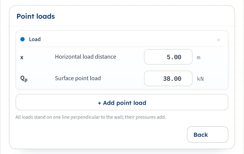
| Field | Symbol | Unit | Default | What to enter |
|---|---|---|---|---|
| Horizontal load distance | x | m · ft | 5.00 | Horizontal distance from the wall to the load, zero or more. In the elastic method a load nearer than 0.30 m (0.9843 ft in US) is calculated at 0.30 m. |
| Surface point load | Qp | kN · tf · kip | 38.00 | The load on the ground surface, zero or more. |
Adding and removing loads
- + Add point load adds a load. It starts a fifth of the wall height beyond the last one (rounded to 0.5 m, and at least 1 m), with the same load: with the example wall it starts at x = 8 m, then 11 m. The cursor moves to its distance box.
- The cross on a card removes that load. It is disabled while only one load is left.
- At three loads the button reads Up to 3 point loads and is disabled.
- All loads stand on one line perpendicular to the wall; their pressures add. Each load has its own colour in the cards, the drawings and the chips.
- After Analyze the add and remove buttons are disabled with the rest of the inputs.
Units
The unit system is chosen in the header and applies to the boxes, the drawings, the results and the report. You can change it before or after Analyze.
| Quantity | SI · kN | SI · tf | US |
|---|---|---|---|
| Length (H, x, L, depths) | m | m | ft |
| Load Qp | kN | tf | kip |
| Resultant PH | kN/m | tf/m | kip/ft |
| Pressure σH | kPa | t/m² | ksf |
Choosing the method
Both methods describe a wall that does not yield, and both give a pressure diagram whose area is PH and whose centroid is at L. They differ in how the distance of the load counts.
| Elastic · rigid wall (default) | Terzaghi–NAVFAC chart | |
|---|---|---|
| Basis | The stress of a point load in an elastic half-space (Boussinesq), doubled for a smooth, unyielding wall by the method of images (Mindlin 1936), with Poisson’s ratio 0.5. | The chart of Terzaghi (1954) as carried by NAVFAC DM-7.02, in two closed forms by the distance ratio m = x/H. |
| Pressure on the load’s section | σH = (3Qp/π) · x²z / R⁵, with R² = x² + z²; the peak is at z = x/2. | With n = z/H: Case 1 (m ≤ 0.4) σH = 0.28 (Qp/H²) n²/(0.16 + n²)³; Case 2 (m > 0.4) σH = 1.77 (Qp/H²) m²n²/(m² + n²)³. |
| Effect of the distance | Counts at every x ≥ xmin = 0.30 m. A load nearer than that is calculated at 0.30 m, and a caution says so. | Counts only beyond 0.4H. A load within 0.4H is taken as if it stood at 0.4H: the same diagram however close it is. |
| Along the wall (Plan, 3D) | The full rigid-wall field, with R² = x² + y² + z²; the peak lies deeper away from the load. | The pressure of the section is reduced by cos²(1.1θ), with θ the plan angle from the load’s perpendicular. |
The two methods against the distance of the load
The table gives PH and L for the module’s example (H = 15 m, Qp = 38 kN) with the load at several distances, each run on the module. The chart keeps one diagram while the load is within 0.4H = 6 m, and then follows the distance; the elastic solution follows the distance everywhere, and grows steeply as the load nears the wall.
| x (m) | Elastic PH | Elastic L | Chart PH | Chart L | Chart case |
|---|---|---|---|---|---|
| 1 | 12.09 | 14.01 | 1.99 | 8.81 | Case 1 |
| 2.5 | 4.82 | 12.59 | 1.99 | 8.81 | Case 1 |
| 5 | 2.34 | 10.59 | 1.99 | 8.81 | Case 1 |
| 6 | 1.91 | 9.94 | 1.99 | 8.81 | Case 1 |
| 6.1 | 1.88 | 9.88 | 1.98 | 8.74 | Case 2 |
| 8 | 1.35 | 8.87 | 1.38 | 7.61 | Case 2 |
| 10 | 1.00 | 8.05 | 0.9755 | 6.74 | Case 2 |
| 15 | 0.5213 | 6.80 | 0.4402 | 5.45 | Case 2 |
With the load at 0.30 m, the nearest the elastic solution takes it, PH is 40.32 kN/m at L = 14.70 m; see Messages for the caution that goes with a load that close.
Which should I pick?
- Use the elastic solution (the default) when the distance of the load matters to you, as in a check of a crane, a stockpile or a truck at different positions: moving the load changes the answer at every distance down to 0.30 m.
- Use the chart when your design basis names the Terzaghi–NAVFAC point-load chart. Its diagram is the one many sheet-pile and trench manuals use; within 0.4H it does not react to the distance.
- Run both. The window opened by the (?) beside a method gives PH and L by both for the current inputs. For the example they are 2.34 kN/m (elastic) and 1.99 kN/m (chart), and the elastic resultant acts higher: 10.59 m against 8.81 m above the base.
Analyze and read the results
Press Analyze. The bar at the foot of the Model tab, which read “Not analysed”, now reads “Analysed — the lateral pressure calculated”; the inputs are locked, and the pressure diagram and the resultant appear on the drawings. Edit inputs unlocks the inputs and clears the results; the bar says the unit system can still be changed while the model is analysed.
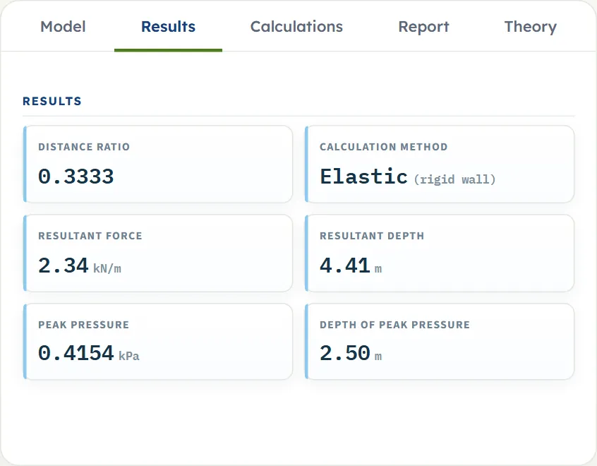
The Results tab shows cards. With one load:
- Distance ratio m = x/H, the ratio the pressure was calculated at. For an elastic load held at 0.30 m a line under the value says “x/H = … as entered · calculated at xmin”.
- Calculation method (Elastic, with “(rigid wall)” beside it) for the elastic solution, or Calculation case (Case 1 for m ≤ 0.4, Case 2 for m > 0.4) for the chart.
- Resultant force PH, in force per metre of wall, at the section of the load.
- Resultant depth, below the ground surface. The height L above the base is H minus this depth, and the Calculations tab gives both.
- Peak pressure σH,max and the Depth of peak pressure.
Several loads
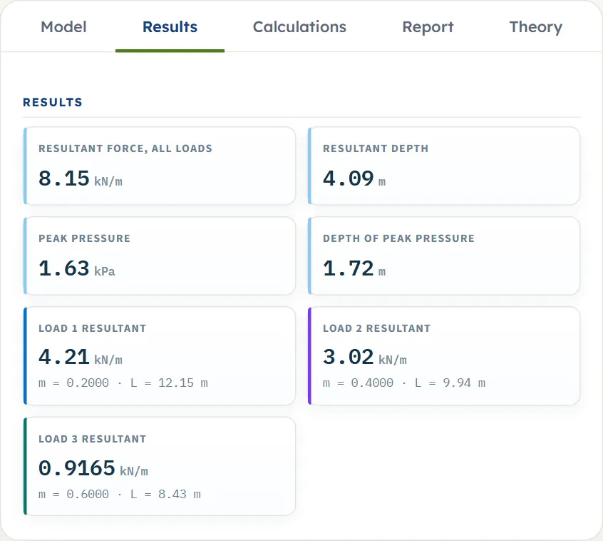
With two or three loads the cards give the Resultant force, all loads, the resultant depth, the peak pressure and its depth for the summed diagram, and then a card for each load, in its colour: its own PH, with its m, its L and, for the chart, its case. The loads add: the total PH is the sum of the loads’ resultants, and the total L is where their moments about the base balance. The peak of the summed diagram can lie between the peaks of the single loads.
What the numbers are
- PH is the force of the surcharge pressure per unit length of wall at the section of the load (along the wall at the load’s own position, y = 0). The Plan and 3D views show how the pressure falls off on either side.
- L is measured up from the base; the card gives the same level as a depth below the ground.
- The resultant is the area of the pressure diagram over the full height of the wall, so it depends on H even when the peak pressure does not (see how each input changes the answer).
The Calculations tab, the report and the theory
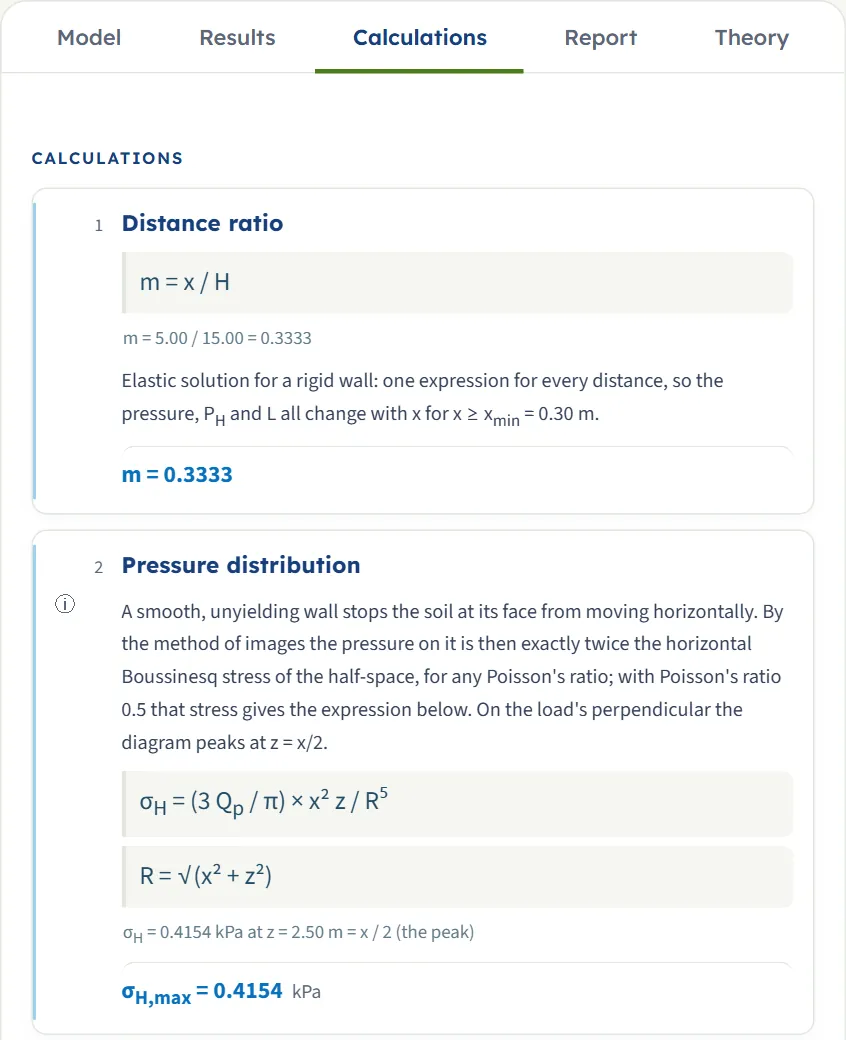
The Calculations tab writes out the working, step by step, with the numbers of your model. After Analyze it has five steps:
- Distance ratio (Distance ratios with several loads) — m = x/H for each load (for the chart, with its case; for an elastic load held at 0.30 m, the ratio it was calculated at).
- Pressure distribution — the equation of the method, the pressure at the depth of the peak, and the peak σH,max . With several loads, the pressure of each load at that depth and their sum.
- Resultant — PH = (Qp/H) × I0, with I0 the dimensionless area of the diagram, and the value of PH; with several loads, one line per load and the sum.
- Location — L = H × I1/I0, with I1 the dimensionless moment about the base, and L above the base and below the surface; with several loads, the balance of moments.
- Plan distribution — the equation for the pressure along the wall (the elastic field with y, or the chart’s cos²(1.1θ)). y and θ are not inputs: the Plan and 3D views sweep them.
Cautions and notes about the run are printed in the Calculations tab where they arise.
The report
The Report tab turns the same working into a summary report. Fill in the cover (Project, Location, Client, Report no., Date, Prepared by (name), Title / qualification, Checked by and optional Notes). The details are kept in this browser. After Analyze, press Save as PDF or Download Word (.docx).
The report has a cover page with the key results, then: 1 Introduction and scope, 2 Input data (the inputs table and the three drawings), 3 Calculation (one part per step), 4 Results, 5 Summary and 6 References. When the run has cautions or notes, an Assumptions and notes section is added after Results, and the Summary and References move down by one. The report is in the unit system shown, and states it with the conversion constants.

The Theory tab explains the method: what the module computes, the two methods, the elastic method, the chart method, the resultant and its location, the pressure in plan and several loads, a worked example and the references.
Worked example: the module’s own example
The module opens on this example, so you can follow the numbers on your own screen.
| Section | Input | Value |
|---|---|---|
| Geometry | Wall height | H = 15 m |
| Method | Calculation method | Elastic · rigid wall |
| Point loads | Distance, load | x = 5 m, Qp = 38 kN |
Step 1: the distance ratio
m = x/H = 5.00/15.00 = 0.3333.
Step 2: the pressure and its peak
On the load’s section the pressure is σH = (3Qp/π) x²z/R⁵ with R² = x² + z². It peaks at z = x/2 = 2.50 m. There R² = 25 + 6.25 = 31.25 m², R⁵ = 5,459.2 m⁵, so
Step 3: the resultant
The area of the diagram over the wall height is PH = (Qp/H) I0, with, for the elastic solution, I0 = [1/m − m²/((1 + m²)√(1 + m²))]/π. For m = 1/3 the bracket is 3 − 0.111111/1.171214 = 2.905131, so I0 = 0.92473 and
Step 4: its height
The moment about the base gives I1 = I0 − 1/(π(1 + m²)√(1 + m²)) = 0.92473 − 0.27178 = 0.65295, so
That is 4.41 m below the ground surface, the “Resultant depth” of the Results tab.
The same load by the chart
With the chart, m = 0.3333 ≤ 0.4, so Case 1 governs and the load is taken as if it stood at 0.4H = 6 m: PH = 1.99 kN/m at L = 8.81 m, and the peak pressure is 0.2737 kPa at 4.24 m, z = √0.08 H. Moving the load anywhere inside 6 m leaves these numbers unchanged.
Three loads
Add two more loads, with x = 3, 6 and 9 m and Qp = 40, 60 and 30 kN, and run the elastic method again. The three loads give PH = 4.21, 3.02 and 0.9165 kN/m, at L = 12.15, 9.94 and 8.43 m. For the first, m = 0.2, I0 = 1.5795 and PH = 40/15 × 1.5795 = 4.21 kN/m. The pressures add, so the total is PH = 4.21 + 3.02 + 0.9165 = 8.15 kN/m, and its height is where the moments about the base balance:
The peak pressure of the summed diagram is 1.63 kPa at 1.72 m. By the chart the same three loads give PH = 6.16 kN/m at L = 8.56 m.
How each input changes the answer
Each row below changes one thing in the example and runs the module again. The numbers are the results the module gives, in the SI · kN system, so you can reproduce any row.
| Change | PH (kN/m) | L (m) | σH,max (kPa) | at depth (m) | What happens |
|---|---|---|---|---|---|
| The default example | 2.34 | 10.59 | 0.4154 | 2.50 | The reference: H = 15 m, x = 5 m, Qp = 38 kN |
| Load at 2.5 m | 4.82 | 12.59 | 1.66 | 1.25 | Closer: the pressure is larger and acts higher |
| Load at 10 m | 1.00 | 8.05 | 0.1039 | 5.00 | Farther: smaller and lower |
| Load at 0.1 m | 40.32 | 14.70 | 115.40 | 0.1500 | Held at 0.30 m; a caution says so |
| Load 76 kN | 4.69 | 10.59 | 0.8309 | 2.50 | Twice the load: everything doubles |
| Wall 10 m | 2.20 | 6.07 | 0.4154 | 2.50 | PH falls because the diagram is cut shorter; the peak does not change |
| Wall 20 m | 2.38 | 15.37 | 0.4154 | 2.50 | PH rises a little; the peak does not change |
| Chart | 1.99 | 8.81 | 0.2737 | 4.24 | Case 1; the same for any x up to 6 m |
| Chart, load at 8 m | 1.38 | 7.61 | 0.1557 | 5.66 | Case 2: the distance counts again |
| Chart, wall 10 m | 2.27 | 5.25 | 0.3986 | 3.54 | 0.4H = 4 m; the load at 5 m is now Case 2 |
What the rows show
- The load scales everything. PH and the pressure are proportional to Qp; L does not depend on it.
- The distance moves the diagram. In the elastic solution the peak sits at z = x/2 and equals 0.2733 Qp/x² (0.4154 kPa at 5 m, 1.66 kPa at 2.5 m); PH falls as the load moves away (12.09, 4.82, 2.34 and 1.00 kN/m at 1, 2.5, 5 and 10 m).
- The wall height changes the resultant, not the peak. In the elastic solution the peak depends on x and Qp only; the height decides how much of the diagram is on the wall, so PH and L change.
- The chart ignores the distance inside 0.4H, and follows it beyond: PH is 1.99 kN/m with the load at 6 m, 1.98 kN/m at 6.1 m and 1.38 kN/m at 8 m.
Messages: stops, cautions and notes
The module tells you in plain words when something prevents the calculation and when a result needs care.
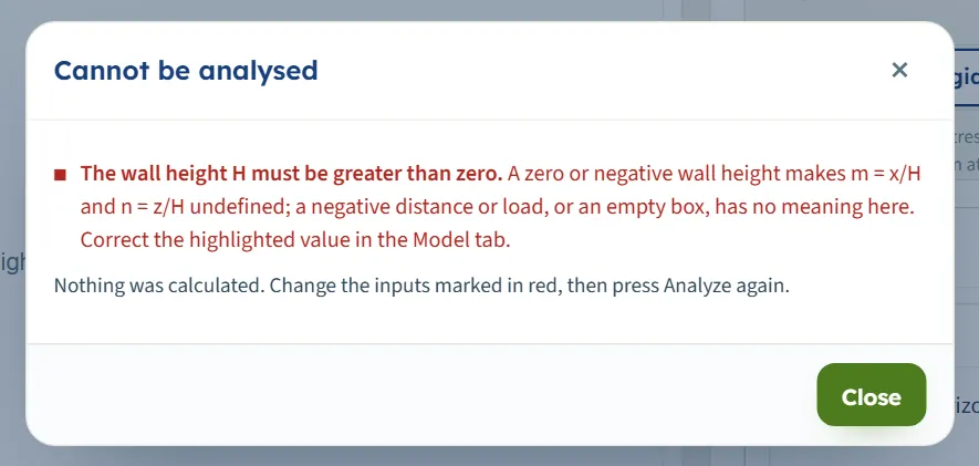
A stop means nothing is calculated. The bar reads “Cannot be analysed” followed by the reason; a red message appears in the Model tab above the bar; the drawings say “Not calculated”; and pressing Analyze opens a window with the message and “Nothing was calculated. Change the inputs marked in red, then press Analyze again.”
| Kind | When | Message and what to do |
|---|---|---|
| Stop | The wall height is zero, negative or empty | “The wall height H must be greater than zero.” A zero or negative wall height makes m = x/H and n = z/H undefined; a negative distance or load, or an empty box, has no meaning here. “Correct the highlighted value in the Model tab.” |
| Stop | A distance is negative or empty | “The horizontal distance x must be zero or more.” (with several loads: “The horizontal distance x₂ of load 2 must be zero or more”.) Correct the value the message names. |
| Stop | A load is negative or empty | “The point load Qₚ must be zero or more.” (with several loads: “The point load of load 2 must be zero or more”.) Several faults are listed together, separated by semicolons. |
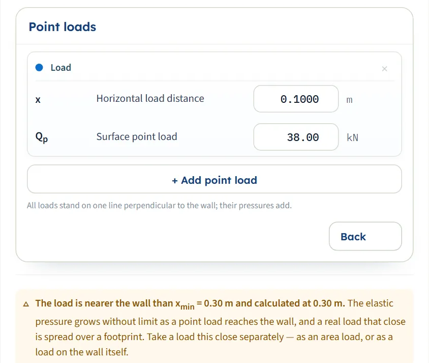
| Caution (amber, in the Model tab) | Elastic method: a load nearer the wall than xmin = 0.30 m | “The load is nearer the wall than xmin = 0.30 m and calculated at 0.30 m. The elastic pressure grows without limit as a point load reaches the wall, and a real load that close is spread over a footprint.” Take a load this close separately, as an area load or as a load on the wall itself. With several loads it names them: “Load 1 is nearer…” or “Loads 1 and 2 are nearer…”. |
| Note (in the Calculations tab and the report) | Chart method: a load within 0.30 m of the wall | “The load is within 0.30 m of the wall. The chart holds any load within 0.4H at 0.4H, so it returns the same pressure however close the load stands.” Take a load this close separately, as above. |
A caution shows in the Model tab under the load cards as soon as the inputs call for it, and again in the Calculations tab and the report; a note shows in the Calculations tab and the report. In the example, a load at 0.1 m by the elastic method:
The Results tab then shows the ratio the load was calculated at (0.0200) and “x/H = 0.006667 as entered · calculated at xmin”, the method card reads “(at xmin)”, and the report gets its Assumptions and notes section.
Good practice and common mistakes
- Measure x from the face of the wall, along the ground, perpendicular to it, to the point where the load acts.
- Treat a spread load as a spread load. A point load is the right idealisation for a footing or a wheel that is small against its distance from the wall. For a load that is wide, or very close, use the Area loads, Strip load or Line load module.
- Say which method your design basis uses. The elastic solution reacts to the distance at every distance; the chart does not inside 0.4H. Run both and keep the one your basis asks for.
- Read PH as a force per metre at the load’s section. Along the wall the pressure falls away (see Plan); the figure is not a total over the wall.
- Use L for the point of application. It is the height of the centroid of the whole diagram, above the base.
- Add the load to the other actions. The module gives the surcharge component only; combine it with the earth and water pressures of your wall analysis.
- Check the units after you switch the system: type values in the units shown beside the boxes.
- Read the cautions and notes. They list what the module assumed for this run, and they are printed in the report.
Frequently asked questions
How do I calculate the lateral pressure on a wall from a point load?
Enter the wall height H, the load Qp and its horizontal distance x from the wall in GeoTerva’s Point load module and press Analyze. The module gives the pressure diagram on the load’s section, its resultant PH in force per metre of wall, the height L of the resultant above the base, and the peak pressure and its depth, by the elastic solution for a rigid wall or by the Terzaghi–NAVFAC chart.
Should I use the elastic method or the chart?
The elastic solution (the default) follows the distance of the load at every distance down to 0.30 m. The chart takes a load within 0.4H as if it stood at 0.4H, so it does not react to the distance there. Use the one your design basis names; the (?) window beside each method gives PH and L by both for your inputs. For the module’s example they are 2.34 kN/m and 1.99 kN/m.
Why does the pressure not change when I move the load closer, with the chart?
The chart holds any load within 0.4H of the wall at 0.4H, so inside that range it returns the same diagram. With H = 15 m the example gives 1.99 kN/m and L = 8.81 m for any x up to 6 m. Switch to the elastic solution if you want the distance to count.
What does the caution about 0.30 m mean?
In the elastic solution the pressure grows without limit as a point load reaches the wall, so a load nearer than xmin = 0.30 m is calculated at 0.30 m, and the module says so. A real load that close is spread over a footprint: take it as an area load or as a load on the wall.
What is PH and where does it act?
PH is the resultant of the surcharge pressure on the wall, the area of the pressure diagram over the wall height, in force per metre of wall (kN/m, tf/m or kip/ft), at the section through the load. It acts at the height L above the base, the centroid of the diagram; the Results tab also gives that level as a depth below the ground.
How many loads can I enter, and where must they be?
Up to three. They all stand on one line perpendicular to the wall, each with its own distance x and load Qp, and their pressures add: the total PH is the sum, and L is where the moments about the base balance. Press + Add point load to add one; the cross on a card removes it.
Can I move the load by dragging it?
Yes, before Analyze: drag the dot at the foot of the load arrow in Elevation, Plan or 3D View. The distance changes in steps of 0.05 of the length unit shown, from 0 to the far edge of the drawing in that view, and the box follows. After Analyze the inputs are locked until you press Edit inputs.
How does the module relate to the earth pressure on the wall?
It gives the surcharge component, the pressure added by the load, which you combine with the earth pressure, the water pressure and the other actions of your wall analysis.
Which module do I use for a line, strip, triangular or uniform load?
The Surcharge Loads family has a module for each: Strip load, Line load, Triangular load, Uniform load, Area loads and Ramp load.
Which units does the module use, and what does the report contain?
SI · kN, SI · tf or US, switched in the header. The report carries the cover, the introduction, the input data with the three drawings, the working, the results, a summary and the references, in the unit system shown, as a PDF or a Word file.