

What the module calculates
Pile on layered soil gives the ultimate axial capacity Qu and the allowable axial capacity Qall of one pile that passes through an arbitrary stack of sand and clay layers. Each layer is typed on its own, and the module works each one by the method for its soil:
- The point bearing Qp follows the soil the tip stands in: a sand tip by Meyerhof, Vesic or Coyle & Castello, a clay tip by Meyerhof (qp = 9cu) or Vesic, and for a bored pile Reese & O’Neill’s expression.
- The skin friction Qs is worked out layer by layer: a sand layer by the K–δ method or Coyle & Castello, a clay layer by the α, λ or β method, each layer with its own coefficients.
- Up to eight layers, a water table, a circular or square pile, driven, bored or jacked, one factor of safety on the total or one on each part.
Use it whenever the profile is not a single soil: sand over clay, clay over sand, a soft layer in dense sand. It also handles a profile that is all sand or all clay, with the same inputs. The one-soil modules, Pile in sand and Pile in clay, are the shorter forms.
What belongs to other modules
- This module treats one pile under an axial compression load, and the results are the resistance of the ground: the weight of the pile is not deducted, as the module says under its results.
- Neighbouring piles are covered by Pile group, and a sideways load by Pile under lateral load.
Before you start: what you need
| What | Where it comes from | Notes |
|---|---|---|
| The profile: layer thicknesses and the type of each layer, sand or clay | Boring logs | The layers must reach at least the pile tip; the module stops if they do not. |
| φ′ for each sand layer, cu for each clay layer | SPT or CPT correlations, tests | A sand layer is asked for φ′ and a clay layer for cu, nothing else about strength. |
| Unit weights γ and γsat | Laboratory or correlations | They give the effective stress through the layers; below the water table γsat − γw is used. |
| Water table depth | Piezometers, borings | Optional. |
| Pile: shape, width or diameter, embedded length, installation | Your design | Installation decides which methods are open and what the module fills in. |
| For a clay layer by the β method: φ′R and OCR | Drained tests on remoulded clay; the stress history | Entered, not correlated: the boxes open at 30° and OCR 1. |
| Factor of safety; applied working load | Your design basis | The module’s hint for the factor is 2.5 to 4. The applied load is optional. |
Quick start in eight steps
- Open the module and choose the units
Open Pile on layered soil from the Piles family and pick SI · kN, SI · tf or US. Open Pile on layered soil.
- Describe the layers, one at a time
In Soil layers, choose Sand or Clay for the layer, fill in its thickness, γ, γsat and φ′ (sand) or cu (clay), and press + Add layer. The module already holds the example’s three layers: click a row to change it, the cross to remove it, then work from the ground surface down; the layers must reach the pile tip.
- Set the groundwater
In Groundwater, choose Present and give the depth, or None.
- Describe the pile
In Pile, choose the shape and the installation (Driven, Bored or Jacked), then enter D and L.
- Choose the method for the point
In Point bearing, pick the method for the soil the tip stands in. The buttons that do not apply to that soil are not offered.
- Choose the method for each layer’s shaft
In Skin friction, every layer has its own method and its own coefficients: K–δ method or Coyle & Castello for sand; α method, λ — extended or β method for clay.
- Set the design values
In Design, enter the factor of safety and, if you want a check, the applied working load.
- Press Analyze and read the answer
Press Analyze. The Results tab gives Qu, Qp, Qs and Qall and the contribution of every layer; Calculations shows every step; Report saves a PDF or Word file.
The screen: three views of the pile
The layout is the one every GeoTerva module shares, described in the workspace guide. The drawing has three views:
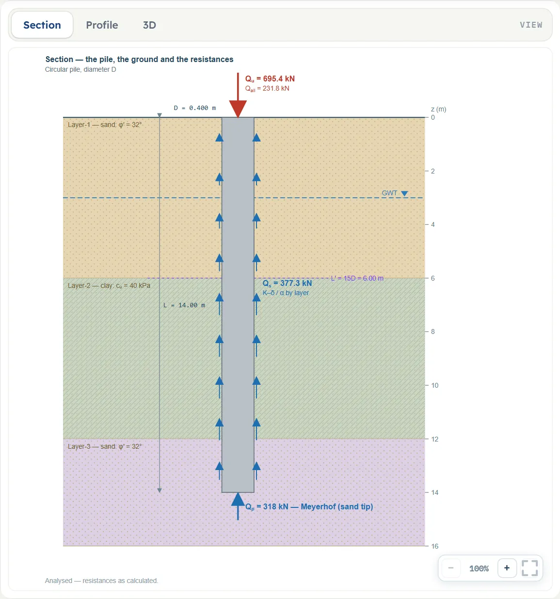
- Section shows the pile through the sand and clay layers (each type in its own colour) with the water table and the resistances Qp, Qs and Qu; the skin-friction arrows follow the unit skin friction. Before you analyse you can drag the water table, a layer base, the pile tip or the side of the pile.
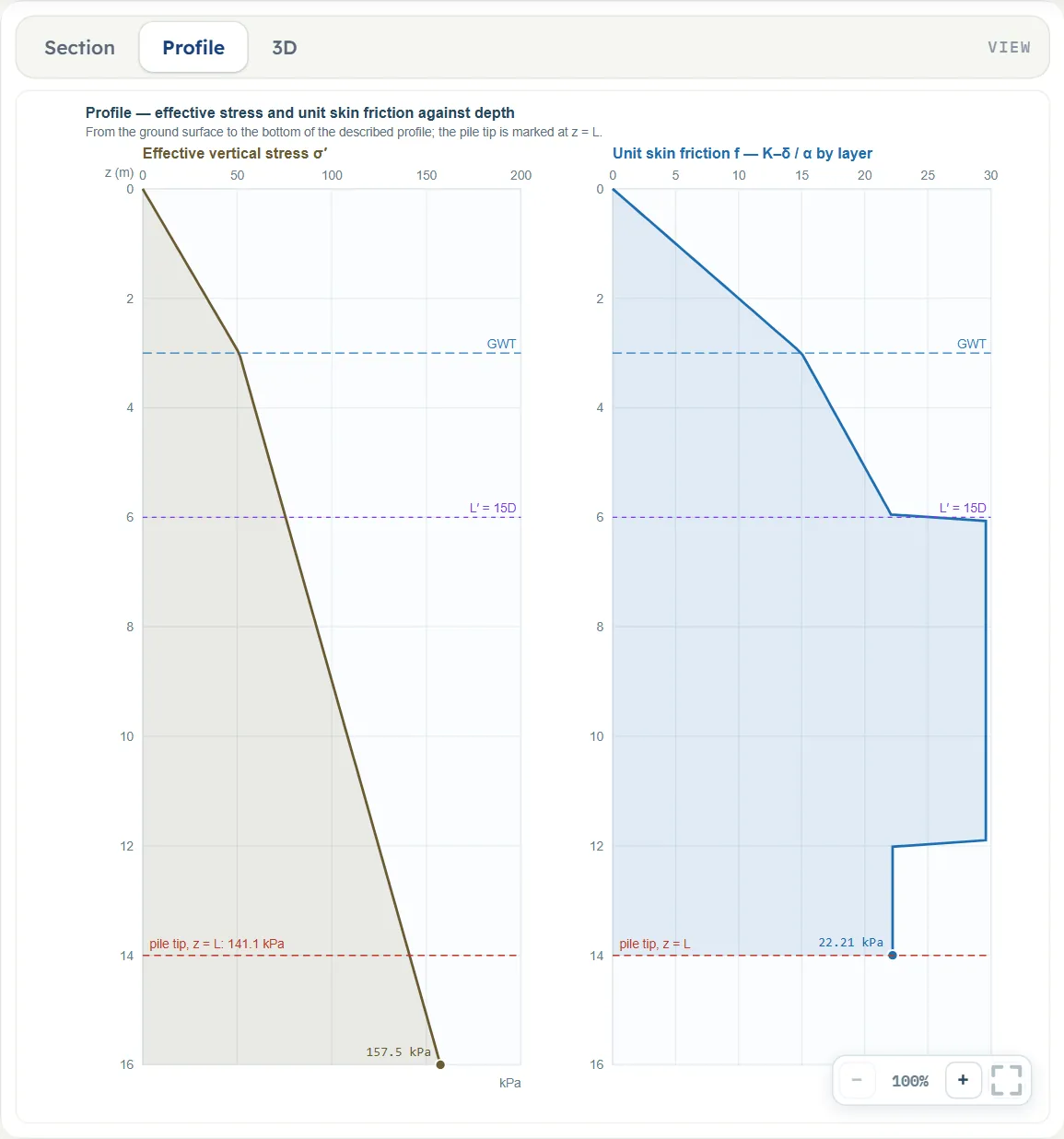
- Profile plots the effective vertical stress σ′ and the unit skin friction f against depth, layer by layer.
- 3D shows the layers and the pile in a block of the ground.
Entering the model, section by section
The Model tab has six sections after Model data. Each opens when you click its title; Next and Back walk you through them, and a (?) opens a help window with a drawing and the formula. Where a unit is shown twice or three times, such as m · ft, the units are those of SI · kN, SI · tf and US in turn, and equal ones are merged. A field marked “filled in” carries a value the module works out; you can type over it.
Soil layers
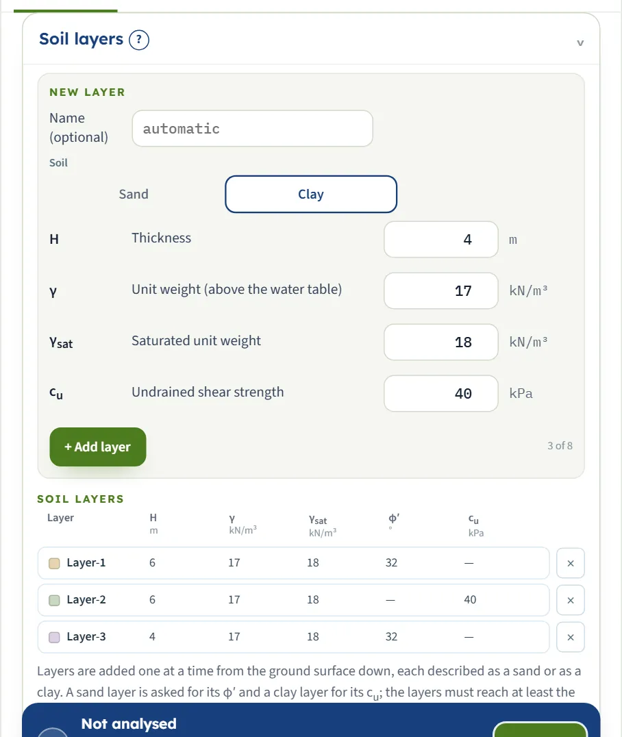
Layers are added one at a time from the ground surface down, each described as a sand or as a clay. A sand layer is asked for φ′ and a clay layer for cu; the box that does not apply is not shown. The values in the table are those of layer 1.
| Field | Symbol | Unit | Default | What to enter |
|---|---|---|---|---|
| Name (optional) | — | — | empty | A name for the layer, for the drawing and the report. Left empty, the layers are called Layer-1, Layer-2 and so on. |
| Thickness | H | m · ft | 6 | Thickness of the layer. The layers together must reach at least the pile tip; the smallest value accepted is 0.1 m. |
| Unit weight (above the water table) | γ | kN/m³ · t/m³ · pcf | 17 | Unit weight above the water table. |
| Saturated unit weight | γsat | kN/m³ · t/m³ · pcf | 18 | Unit weight below the water table; below it the module uses γsat − γw. |
| Friction angle | φ′ | ° | 32 | Effective friction angle of a sand layer, at least 20°. Meyerhof’s chart is drawn from 20° to 45°; above 45° the end value is held at the tip layer and a warning says so. Shown when the layer is Sand. |
| Undrained shear strength | cu | kPa · kg/cm² · psf | 40 | Undrained shear strength of a clay layer, at least 1 kPa. Shown when the layer is Clay. |
Groundwater
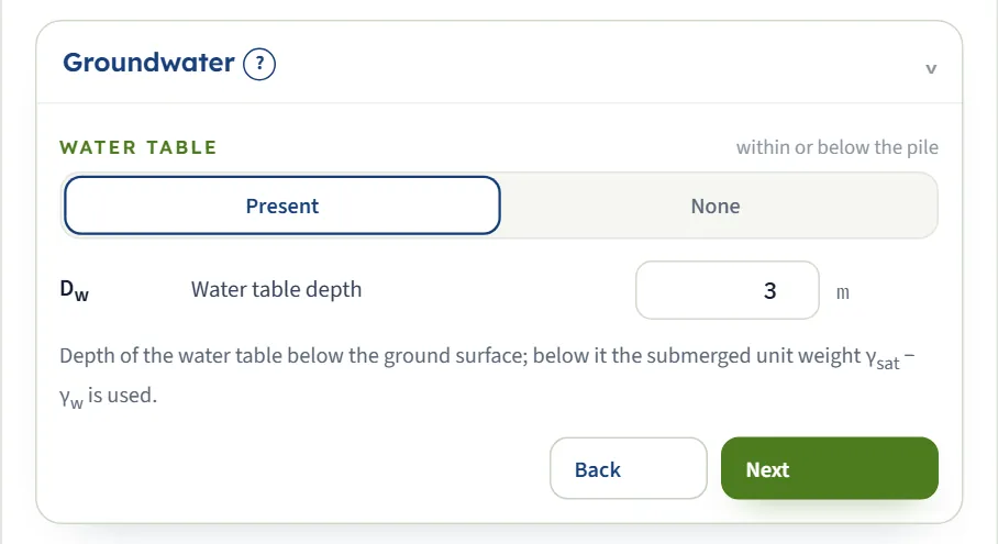
Choose whether there is a water table within the pile length and give its depth. Below it the module uses the submerged unit weight γsat − γw for the effective stress.
| Choice | Options | Default |
|---|---|---|
| Water table within or below the pile | Present None | Present |
| Field | Symbol | Unit | Default | What to enter |
|---|---|---|---|---|
| Water table depth | Dw | m · ft | 3 | Depth of the water table below the ground surface, 0 or more. Shown when the water table is present. |
Pile
The shape and the installation are choices; the width and the length are numbers.
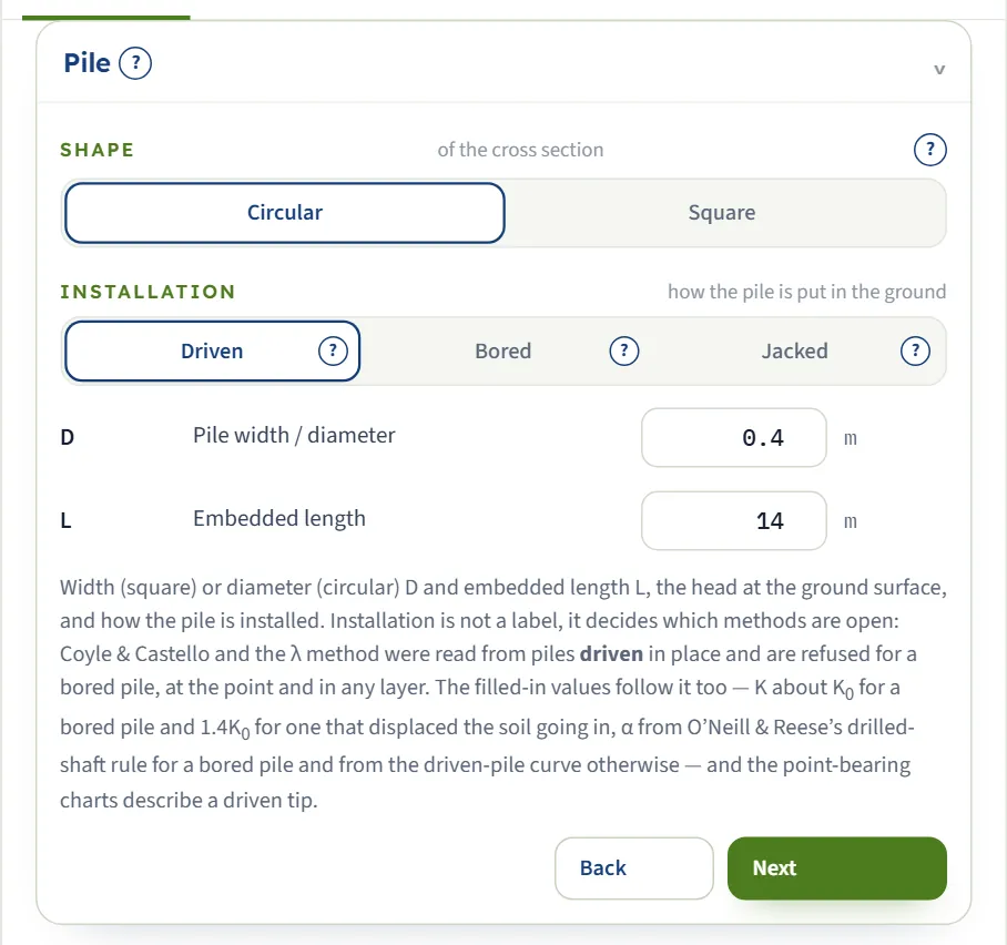
| Choice | Options | Default |
|---|---|---|
| Shape of the cross section | Circular Square | Circular |
| Installation how the pile is put in the ground | Driven Bored Jacked | Driven |
| Field | Symbol | Unit | Default | What to enter |
|---|---|---|---|---|
| Pile width / diameter | D | m · ft | 0.4 | Width of a square pile or diameter of a circular one. |
| Embedded length | L | m · ft | 14 | Embedded length from the ground surface to the tip; the head is at the ground surface. |
Point bearing
The tip is worked out by the soil it ends in. Sand tip: Meyerhof, Vesic (it asks for m) or Coyle & Castello (it fills in N*q). Clay tip: Meyerhof gives qp = 9cu and Vesic builds N*c from the rigidity index; Coyle & Castello is a sand correlation, so that button is not offered while the tip is in clay. For a bored pile with a clay tip Reese & O’Neill’s drilled-shaft expression is offered; it averages cu over the 2D below the base, so that depth has to be clay.
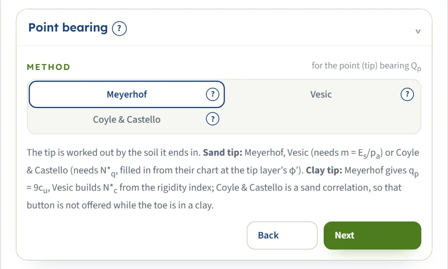
| Choice | Options | Default |
|---|---|---|
| Method for the point (tip) bearing Qp | Meyerhof Vesic Coyle & Castello Reese & O’Neill | Meyerhof |
| Field | Symbol | Unit | Default | What to enter |
|---|---|---|---|---|
| Stiffness ratio of the sand at the tip | m | — | 250 | The stiffness ratio Es/pa of the sand at the tip: about 100–200 loose, 200–500 medium dense, 500–1000 dense. Used only when the tip layer is sand and Vesic is selected. Shown when point-bearing method is Vesic. |
| Coyle & Castello N*q (chart value) | N*q(CC) | — | filled in | Read from the Coyle & Castello chart for the pile’s L/D and φ′ of the tip layer, and kept up to date; type over it or empty the box to get the chart value back. Shown when point-bearing method is Coyle & Castello. |
Skin friction
Every layer chooses its own method and carries its own numbers, named after the layer they belong to. A sand layer: the K–δ method (its own K and δ′, with σ′ held constant below L′ = 15D of the whole pile) or Coyle & Castello (its own chart-read K, δ′ = 0.8φ′, the mean σ′ of that layer). A clay layer: the α method (its own adhesion factor on cu), the λ method (λ read at the pile’s embedded length and applied to that layer’s own mean σ′ and cu) or the β method (its own φ′R and OCR).
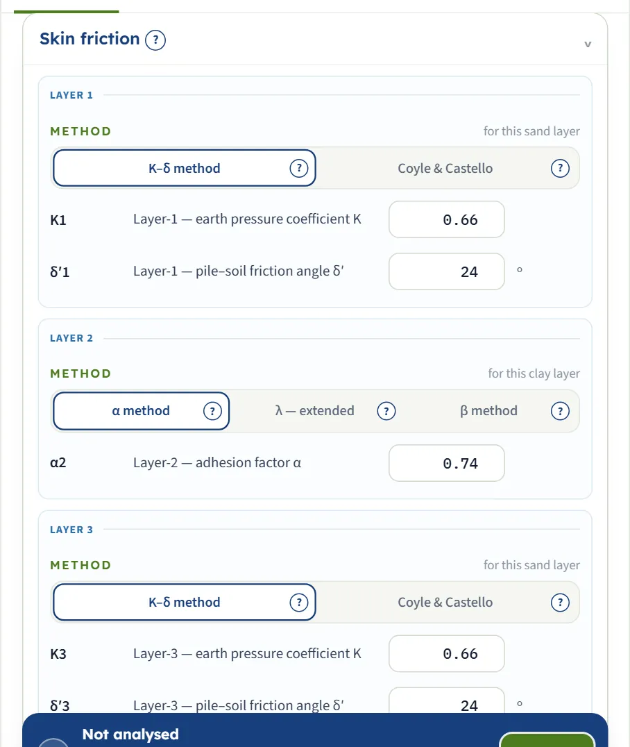
| Layer is | Methods offered | Default |
|---|---|---|
| Sand | K–δ method Coyle & Castello | K–δ method |
| Clay | α method λ — extended β method | α method |
| Field | Symbol | Unit | Default | What to enter |
|---|---|---|---|---|
| Earth pressure coefficient K | K | — | filled in | Earth-pressure coefficient on the shaft in this sand layer. Filled in as K0 = 1 − sin φ′ for a bored pile and 1.4K0 for a driven or jacked one; editable. Shown when the layer is Sand and method is K–δ method. |
| Pile–soil friction angle δ′ | δ′ | ° | filled in | Friction angle between the pile and this sand layer; filled in as 0.75φ′. Shown when the layer is Sand and method is K–δ method. |
| Coyle & Castello K | K(CC) | — | filled in | Coyle & Castello’s coefficient for this sand layer, read from their chart at the layer’s φ′ and the pile’s L/D; the interface friction is 0.8φ′. Shown when the layer is Sand and method is Coyle & Castello. |
| Adhesion factor α | α | — | filled in | Adhesion factor of this clay layer. Filled in from cu/pa by the rule that belongs to the installation (a driven-pile curve, or 0.55 falling to 0.45 for a bored pile); editable. Shown when the layer is Clay and method is α method. |
| Remoulded drained friction angle | φ′R | ° | 30 | Remoulded drained friction angle of this clay layer, for the β method; the box opens at 30°. Shown when the layer is Clay and method is β method. |
| Overconsolidation ratio | OCR | — | 1 | Overconsolidation ratio of this clay layer, for the β method; the box opens at 1. Shown when the layer is Clay and method is β method. |
Design
One factor of safety on the sum, or a separate factor on each part: Qall = Qp/FSp + Qs/FSs. An applied working load is optional.
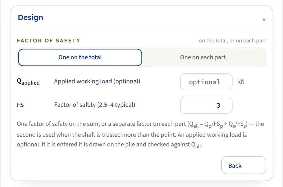
| Choice | Options | Default |
|---|---|---|
| Factor of safety on the total, or on each part | One on the total One on each part | One on the total |
| Field | Symbol | Unit | Default | What to enter |
|---|---|---|---|---|
| Applied working load (optional) | Qapplied | kN · tf · kip | empty | The working load the pile has to carry. Optional: if it is entered it is drawn on the pile and checked against Qall. |
| Factor of safety (2.5–4 typical) | FS | — | 3 | One factor of safety on Qu; the module’s hint is 2.5 to 4. Shown when factor of safety is One on the total. |
| Factor of safety on the point resistance | FSp | — | 3 | Factor of safety on the point resistance (one factor on each part). Shown when factor of safety is One on each part. |
| Factor of safety on the skin friction | FSs | — | 1.5 | Factor of safety on the skin friction. Shown when factor of safety is One on each part. |
How the layers combine
The methods themselves are those of the one-soil modules, explained in the manuals of Pile in sand and Pile in clay. What this module adds is the rule for combining them:
| Part | Rule | Consequence |
|---|---|---|
| Point bearing | Worked by the soil the tip stands in, whatever lies above it. | A strong sand above a soft clay tip gives a clay Qp: the sand does not help the tip. With the example’s tip in sand, Qp = 318 kN; make the tip layer clay and it is 45 kN. |
| Tip on a boundary | A tip exactly on a layer boundary bears on the layer below it. | The module says which layer it took; the layer above contributes shaft friction only. |
| Effective stress | Continuous through all the layers, with the unit weights of each and the water table. | σ′ at any depth includes everything above it, so a deep layer of any type has a high σ′. |
| K–δ critical depth | L′ = 15D of the whole pile, from the ground surface. | In a K–δ sand layer, σ′ is held at its value at L′ at every depth below L′. |
| Shaft | Summed over the layers the pile passes through, each by its own method. | The Results tab lists each layer’s skin friction and its share. |
Which should I pick?
- Sand layers: the K–δ method is the default; use Coyle & Castello when you want the load-test charts and the pile is driven.
- Clay layers: the α method is the default and works on cu alone. Use β when you hold effective-stress parameters. Treat the λ extension as an estimate.
- The point: Meyerhof for either soil is the default; Vesic adds stiffness (m for sand, the rigidity index for clay).
- Compare by changing one method at a time and keeping each run with Quick Save…; the what-if table shows the spread on the example.
Analyze and read the results
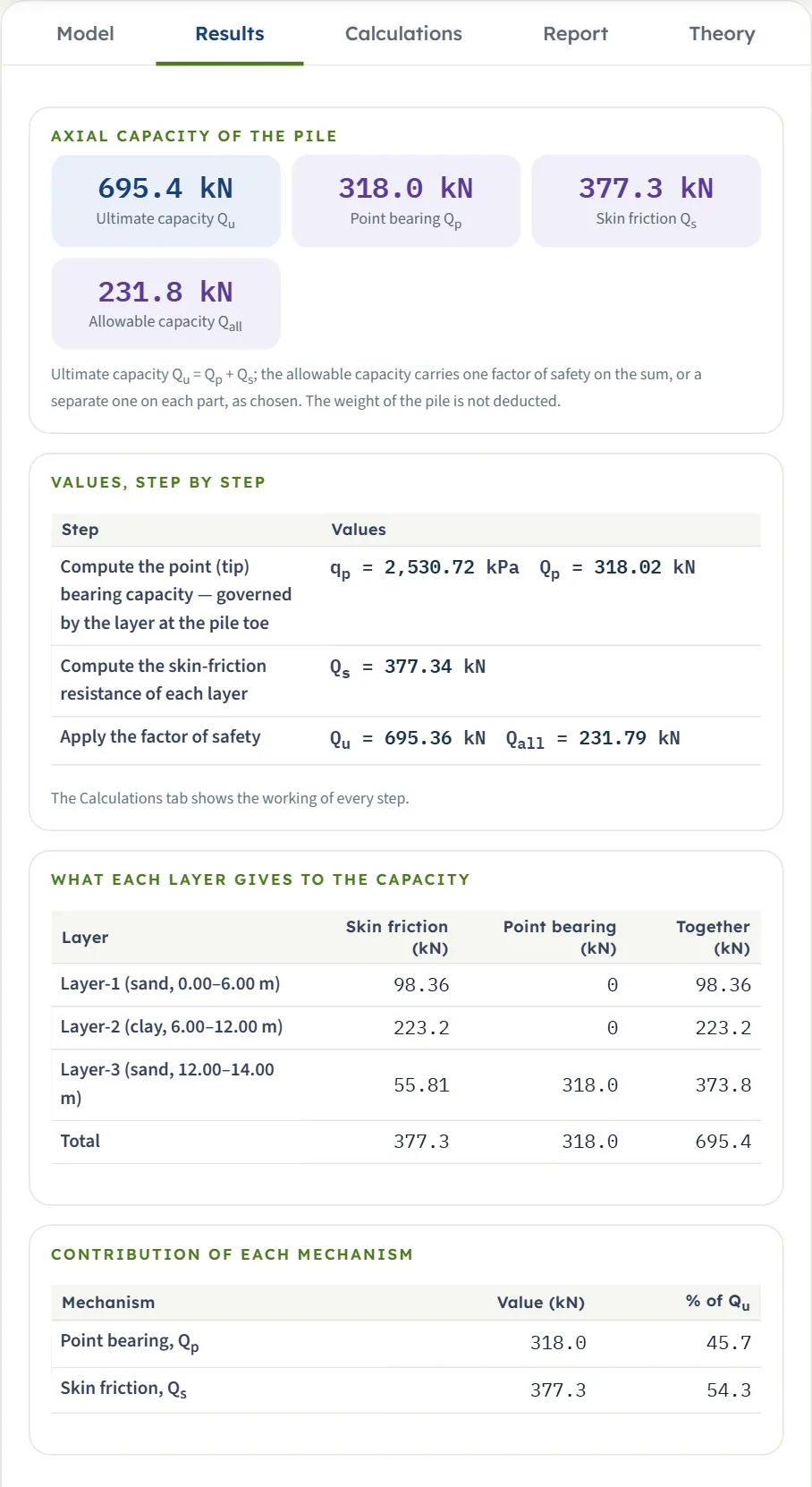
Press Analyze. The bar reports the run, the inputs lock, and the Results tab shows four blocks.
- Axial capacity of the pile. Cards for Qu, Qp, Qs and Qall.
- Values, step by step. The point bearing (qp, Qp), the skin friction of the layers (Qs) and the factor of safety.
- What each layer gives to the capacity. Every layer with its type and depth range, its skin friction and, for the tip layer, the point bearing.
- Contribution of each mechanism. The share of the point and of the shaft in Qu.
Checking an applied load
If you enter an applied working load, the Results tab adds the ratio Qapplied/Qall and a verdict in words: PASS when the load is within the allowable capacity, FAIL when it exceeds it, with a warning that advises lengthening or widening the pile, using more piles, or revisiting the factors of safety.
The Calculations tab and the report
The Calculations tab starts with Given and what is sought, then:
- Compute the point (tip) bearing capacity — governed by the layer at the pile toe. It says which soil the tip is in and the method that follows from it.
- Compute the skin-friction resistance of each layer. Every layer by its own method, with its own numbers.
- Apply the factor of safety — Qu and Qall.
- Check the applied working load, when one was entered.
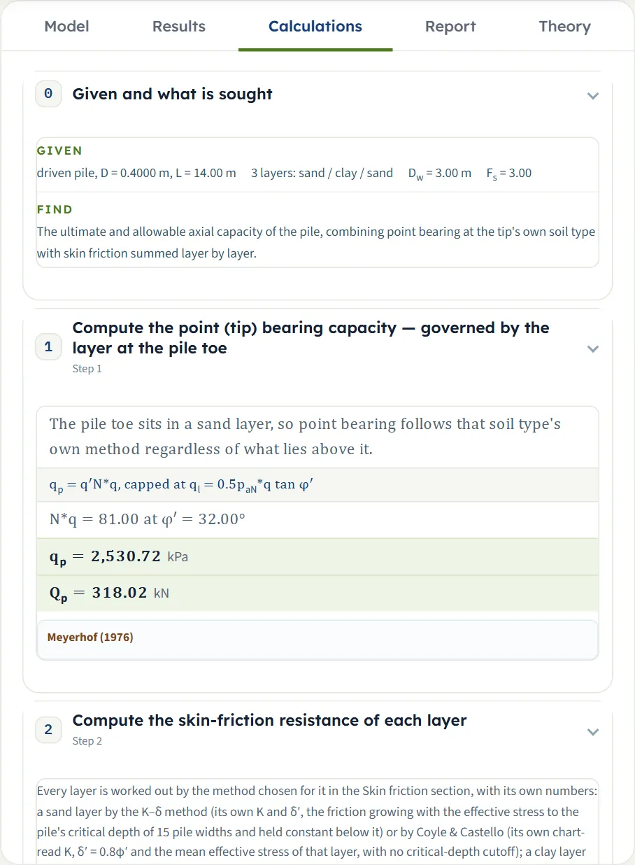
The Report tab fills in a cover and saves the same working as a PDF or a Word file (1 Introduction and scope, 2 Input data, 3 Calculation, 4 Results, then 5 Assumptions and notes when the run has any, and the Summary and References), with the units line. The Theory tab explains a pile through several layers, the effective stress through them, the rules over a sand and over a clay layer, the bored-pile procedure and a worked example.
Worked example: the module’s own example
The module opens on this example; Reset to defaults brings it back.
| Layer | Soil | Thickness H | Strength | γ / γsat | Shaft method |
|---|---|---|---|---|---|
| Layer-1 | Sand | 6 m | φ′ = 32° | 17 / 18 kN/m³ | K–δ |
| Layer-2 | Clay | 6 m | cu = 40 kPa | 17 / 18 kN/m³ | α |
| Layer-3 | Sand | 4 m | φ′ = 32° | 17 / 18 kN/m³ | K–δ |
Water table at 3 m; circular driven pile, D = 0.4 m, L = 14 m (the tip is in Layer-3, 2 m below the clay); Meyerhof for the point; one factor of safety FS = 3. The module fills in K = 0.66 and δ′ = 24° for the sand layers and α = 0.74 for the clay.
Point bearing
The tip is in sand, so the point follows Meyerhof’s sand method with φ′ = 32° of Layer-3. N*q = 81.00; the effective stress at the tip is 17 × 3 + (18 − 9.81) × 11 = 141.09 kPa, so σ′ N*q = 11,428 kPa, far above the limit ql = 0.5 × 100 × 81 × tan 32° = 2,530.72 kPa, which governs. With Ap = π × 0.4²/4 = 0.1257 m², Qp = 318.02 kN.
Skin friction, layer by layer
The perimeter is π × 0.4 = 1.2566 m, and the critical depth is L′ = 15D = 6 m of the whole pile.
| Layer | Depth (m) | How it is worked | Qs (kN) |
|---|---|---|---|
| Layer-1, sand | 0–6 | f = 0.66 tan 24° σ′ over the whole 6 m (σ′ = 51 kPa at the water table, 75.57 kPa at 6 m): 1.2566 × 0.66 tan 24° × 266.36 | 98.36 |
| Layer-2, clay | 6–12 | α cu × perimeter × length = 0.74 × 40 × 1.2566 × 6 | 223.18 |
| Layer-3, sand | 12–14 | σ′ is held at its value at L′ = 6 m: f = 0.66 tan 24° × 75.57 = 22.21 kPa; × 1.2566 × 2 m | 55.81 |
| Total Qs | 377.3 |
Capacity
Qu = 318.02 + 377.34 = 695.36 kN; with FS = 3, Qall = 231.79 kN. The point carries 45.7 % and the shaft 54.3 %.
How each input changes the answer
Each row changes one thing in the example and runs the module again. The numbers are the results the module gives, in kN.
| Change | Qp | Qs | Qu | Qall | Why |
|---|---|---|---|---|---|
| The default example | 318.0 | 377.3 | 695.4 | 231.8 | The reference |
| Point bearing by Vesic (sand tip) | 632.8 | 377.3 | 1,010 | 336.7 | Stiffness enters through m = 250 |
| Point bearing by Coyle & Castello (sand tip) | 585.1 | 377.3 | 962.4 | 320.8 | N*q from the chart, no limit |
| Sand layer 1 by Coyle & Castello | 318.0 | 349.6 | 667.6 | 222.5 | Only Layer-1 changes |
| Clay layer 2 by the λ method | 318.0 | 438.0 | 756.1 | 252.0 | A caution: the layer-by-layer λ is an extension |
| Clay layer 2 by the β method | 318.0 | 372.1 | 690.1 | 230.0 | At-rest K; a note says it is on the safe side |
| Bored pile | 318.0 | 275.7 | 593.7 | 197.9 | K = K0 = 0.47 in the sand, α = 0.55 in the clay; the top 1.5 m and bottom 1D are left out only of clay layers worked by α, and here nothing is cut |
| Jacked pile | 318.0 | 377.3 | 695.4 | 231.8 | Same as driven here |
| Layer-3 made clay (tip in clay) | 45.24 | 395.9 | 441.2 | 147.1 | qp = 9cu = 360 kPa: the tip is in clay |
| No water table | 318.0 | 411.5 | 729.5 | 243.2 | Higher σ′ everywhere |
| Pile 10 m long (tip in the clay) | 45.24 | 247.1 | 292.4 | 97.46 | The point is clay: 9cu |
| Pile 16 m long (tip at the base of the profile) | 318.0 | 433.2 | 751.2 | 250.4 | A note: the deepest layer is taken to continue below the tip |
| Diameter 0.6 m | 715.5 | 593.2 | 1,309 | 436.3 | Larger tip and perimeter, and L′ = 15D = 9 m |
| Square section | 404.9 | 480.5 | 885.4 | 295.1 | Larger area and perimeter |
| Factor of safety on each part | 318.0 | 377.3 | 695.4 | 357.6 | FSp = 3 and FSs = 1.5 |
| Friction angle of Layer-3 = 36° | 766.9 | 377.7 | 1,145 | 381.5 | N*q at the tip rises |
| Clay layer 2: cu = 60 kPa | 318.0 | 434.6 | 752.7 | 250.9 | Only the clay shaft changes |
Cases that the module does not run, such as Coyle & Castello in a layer of a bored pile, or a pile longer than the layers, stop with a message (see Messages).
Messages: stops, warnings and notes
The module says in plain words when something prevents the calculation, when a result needs care, and what it assumed.
| Kind | When | Message and what to do |
|---|---|---|
| Stop (brown bar, “Cannot analyse”) | The layers do not reach the pile tip | “The layers must reach the pile tip. They reach 16.00 m, the pile is 17.00 m long.” Add a layer, or thicken the last one. |
| Stop | Coyle & Castello for a bored pile, at the point or in a sand layer | “Change the skin-friction method of Layer-1. Coyle & Castello is calibrated on piles DRIVEN in sand; a bored pile is outside it.” Use the K–δ method in sand. |
| Stop | The λ method in a clay layer of a bored pile | The λ method was read from driven piles. Use the α or β method. |
| Stop | Vesic at a clay tip where cu is below the start of the correlation | Use Meyerhof for the point (qp = 9cu). |
| Stop | Reese & O’Neill (bored pile) when the 2D below the base reaches into a sand layer | “…so that depth has to be clay: here it reaches into Layer-3, which has no undrained strength.” Use Meyerhof or Vesic for the point, or take the pile deeper into the clay. |
| Stop (input error) | A value below the smallest the field accepts | For example φ′ below 20° in a sand layer. Correct the value; the row of the layer is outlined in red. |
| Warning | Coyle & Castello, or the λ method, for a jacked pile | Read the result as an estimate, or use the K–δ or the α method. |
| Warning | The λ method in a clay layer | “The λ method is applied layer by layer here, which is an extension of it.” Read the λ layers as an estimate, or use α or β. |
| Warning | An applied load larger than Qall | “The pile does not carry the applied load — 129.4% of Qall.” Lengthen or widen the pile, use more piles, or revisit the factors of safety. |
| Warning | K too high for a bored pile (K above 1.25K0 of the layer) | Boring displaces nothing, so K stays near K0 = 1 − sin φ′. Use K ≈ K0, or say why this shaft carries more. |
| Warning | φ′ above 45° in a sand layer | Meyerhof’s chart is drawn from 20° to 45° only; beyond it the end value is held. |
| Note | K well above 1.8K0 for a driven or jacked pile | The range of K for displacement piles is a guide; keep the value if a load test or local practice supports it. |
| Note | The tip exactly on a layer boundary | The point bearing is worked from the layer below the boundary; the layer above gives shaft friction only. |
| Note | The profile ends less than 2D below the tip | The deepest layer is taken to continue below, with the same properties. |
| Note | A bored pile | The drilled-shaft α is used in clay (no friction over the top 1.5 m and the bottom 1D); the friction angle at a sand tip is taken to describe the sand after drilling, and a clay base is taken as clean and undisturbed; no reduction is applied for the bored construction. |
| Note | The β method for a driven or jacked pile | Computed with the at-rest K = 1 − sin φ′R, which is on the safe side. |
| Note | Coyle & Castello beyond their charts | The coefficients are projected beyond L/D = 70 (N*q) or 36.1 (K); the boxes stay editable. |
The Warnings (or Notes) button on the green bar lists them after a run. Most are printed in the report in an Assumptions and notes section; the K cautions and the applied-load warning stay on screen.
Good practice and common mistakes
- Type each layer correctly. Sand takes φ′, clay takes cu; a layer typed wrongly changes both the shaft and, at the tip, the point bearing.
- Look at the tip layer. The point bearing answers only to it. The point is worked from the layer the tip stands in (with Reese & O’Neill, from the mean cu over the 2D below the base); a softer layer beneath the tip does not change it.
- Match the installation to the pile. It decides which methods are open and what K and α are filled in with.
- Read the layer table. It shows which layers carry the shaft; in the example the clay carries most of it.
- Remember the whole-pile critical depth. In the K–δ method L′ = 15D counts from the ground surface, so a deep sand layer gets the value at L′.
- Run more than one method and keep each run with Quick Save….
- Read the notes. They list what the module assumed.
Frequently asked questions
How do I calculate the capacity of a pile in layered soil?
The ultimate capacity is the point bearing plus the skin friction, Qu = Qp + Qs. With layered soil the skin friction is summed over the layers, each by the method for its soil, and the point bearing follows the soil the tip stands in. In GeoTerva’s Pile on layered soil module you type each layer as sand or clay, choose a method for each, press Analyze, and read Qp, Qs, Qu, Qall and the contribution of every layer.
Which soil governs the point bearing?
The soil the tip stands in. A strong layer above a soft tip does not help the tip. If the tip is exactly on a boundary, it bears on the layer below it, and the module says so.
Can I mix methods in one pile?
Yes. Every layer chooses its own: K–δ or Coyle & Castello in a sand layer, α, λ or β in a clay layer, and the point has its own method for the soil at the tip.
What does the K–δ critical depth do in a layered profile?
The critical depth L′ = 15D counts from the ground surface for the whole pile. Sand layers deeper than L′ get the unit friction at L′, held constant. In the example the deep sand layer gets 22.2 kPa, not the larger value its own effective stress would give. A Coyle & Castello layer has no such cut-off.
Why is the λ method called “extended” here?
The λ method was written as one average over the whole embedded length. The module applies it layer by layer, reading λ at the pile’s length and using each clay layer’s own mean stress and strength. It warns you and suggests the α or β method for a layered profile.
Can I use Coyle & Castello for a bored pile in layered soil?
No. It was read from driven piles, so the module stops and asks you to use the K–δ method in sand and Meyerhof or Vesic at the point. A jacked pile gets a caution.
How many layers can I enter?
Up to eight, each typed as sand or clay. They must reach at least the pile tip.
What does the water table change?
Below it the module uses γsat − γw for the effective stress, which lowers the shaft friction in the K–δ, Coyle & Castello, λ and β methods. The α method works on cu and does not change. In the example removing the water table raises Qs from 377 kN to 412 kN.
Is there a free version I can try?
The module opens on a complete example, and a limited version also opens on the Try it page without an account.