

What the module calculates
Pile in clay gives the ultimate axial capacity Qu and the allowable axial capacity Qall of one pile in clay, loaded undrained. As for every pile in the family, the ultimate capacity is what the tip carries plus what the shaft carries:
Qp is the point bearing, worked out on the undrained strength cu of the clay at the tip; Qs is the skin friction, worked out layer by layer. You choose the method for the point and the method for the shaft independently, and can put one factor of safety on the sum or one on each part.
What you can describe
- A ground of up to eight clay layers, each with its thickness, undrained shear strength cu, unit weights and, for the β method, its overconsolidation ratio OCR, and a water table.
- A circular or square pile, driven, bored or jacked, of width or diameter D (at least 0.05 m) and embedded length L (at least 0.5 m).
- Three point-bearing methods: Meyerhof (Qp = 9cuAp), Vesic (the factor N*c from the rigidity index) and, for a bored pile, Reese & O’Neill’s drilled-shaft expression.
- Three skin-friction methods: the α method, the λ method and the β method.
What belongs to other modules
- This module treats one pile under an axial compression load. Neighbouring piles are covered by Pile group, and a sideways load by Pile under lateral load.
- The results are the resistance of the ground: the weight of the pile is not deducted, as the module says under its results.
- The layers here are clay. For sand, or for a profile that mixes sand and clay, use Pile in sand or Pile on layered soil.
Before you start: what you need
| What | Where it comes from | Notes |
|---|---|---|
| The clay profile: layer thicknesses | Boring logs | The layers must reach at least the pile tip; the module stops if they do not. |
| Undrained shear strength cu of each layer | Unconfined or triaxial tests, vane tests, correlations | Used by the α and λ methods and by the point bearing (the strength of the tip layer governs Qp); the β method does not use it. |
| Unit weights γ and γsat | Laboratory or correlations | They give the effective stress used by the λ and β methods. The α method works on cu alone. |
| Water table depth | Piezometers, borings | Below it the submerged unit weight γsat − γw is used for the effective stress (λ and β methods). |
| For the β method: remoulded friction angle φ′R and OCR of each layer | Drained tests on remoulded clay; the stress history | They describe your clay, so you enter them: φ′R opens at 30° and OCR at 1 (the example’s Clay-3 has 2). |
| Pile: shape, width or diameter, embedded length, installation | Your design | Installation decides which methods are open and what the filled-in values are. |
| Factor of safety; applied working load | Your design basis | The module’s hint for the factor is 2.5 to 4. The applied load is optional. |
Quick start in eight steps
- Open the module and choose the units
Open Pile in clay from the Piles family and pick SI · kN, SI · tf or US in the header. Open Pile in clay.
- Describe the clay layers
In Clay layers, fill in the New layer form (thickness, cu, γ, γsat, and OCR for the β method) and press + Add layer; repeat from the ground surface down. The module already holds the example’s three layers: click a row to edit it, the cross to remove it, then add the rest. The layers must reach the pile tip.
- Set the groundwater
In Groundwater, choose Present and give the depth, or None.
- Describe the pile
In Pile, choose the shape and the installation (Driven, Bored or Jacked), then enter D and L.
- Choose the method for the point
In Point bearing, pick Meyerhof, Vesic or, for a bored pile, Reese & O’Neill.
- Choose the method for the shaft
In Skin friction, pick the α method, the λ method (driven piles) or the β method. The α of each layer is filled in; φ′R appears in the Skin friction section and OCR in the layer form (click a row of the table to see it); both are yours to enter.
- Set the design values
In Design, enter the factor of safety and, if you want a check, the applied working load.
- Press Analyze and read the answer
Press Analyze. The Results tab gives Qu, Qp, Qs and Qall and what each layer contributes; Calculations shows every step; Report saves a PDF or Word file.
The screen: three views of the pile
The layout is the one every GeoTerva module shares, described in the workspace guide. The drawing has three views:
- Section shows the pile in the clay layers with the water table and the resistances Qp, Qs and Qu; the skin-friction arrows follow the unit skin friction of each layer. Before you analyse you can drag the water table, a layer base, the pile tip or the side of the pile.
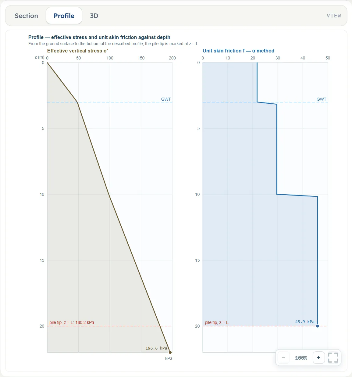
- Profile plots the effective vertical stress σ′ and the unit skin friction f against depth.
- 3D shows the pile in a block of the ground with the layers and the water table.
Entering the model, section by section
The Model tab has six sections after Model data. Each opens when you click its title; Next and Back walk you through them, and a (?) opens a help window with a drawing and the formula. Where a unit is shown twice or three times, such as m · ft, the units are those of SI · kN, SI · tf and US in turn, and equal ones are merged. A field marked “filled in” carries a value the module works out; you can type over it.
Clay layers
Up to eight layers from the ground surface down. The shaft is summed over every layer the pile passes through; the point bearing answers to the layer at the tip. The values in the table are those of layer 1.
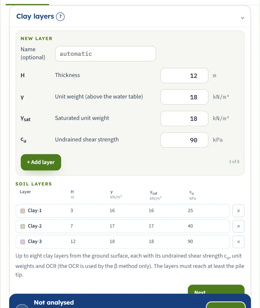
| Field | Symbol | Unit | Default | What to enter |
|---|---|---|---|---|
| Name (optional) | — | — | empty | A name for the layer, for the drawing and the report. Left empty, the layers are called Clay-1, Clay-2 and so on. |
| Undrained shear strength | cu | kPa · kg/cm² · psf | 25 | Undrained shear strength of the layer, at least 1 kPa. The tip layer’s value gives the point bearing; every layer’s value enters the α and λ shaft methods. |
| Unit weight (above the water table) | γ | kN/m³ · t/m³ · pcf | 16 | Unit weight of the clay above the water table. |
| Saturated unit weight | γsat | kN/m³ · t/m³ · pcf | 16 | Unit weight below the water table; below it the module uses γsat − γw for the effective stress. |
| Thickness | H | m · ft | 3 | Thickness of the layer. The layers together must reach at least the pile tip; the smallest value accepted is 0.1 m. |
| Overconsolidation ratio | OCR | — | 1 | Overconsolidation ratio of the layer, at least 1. Used by the β method only. Shown when skin-friction method is β method. |
Groundwater
Choose whether there is a water table within the pile length and give its depth. Below it the effective stress uses the submerged unit weight. It matters for the λ and β methods, which work on effective stress; the α method works on cu alone and does not change with the water table.
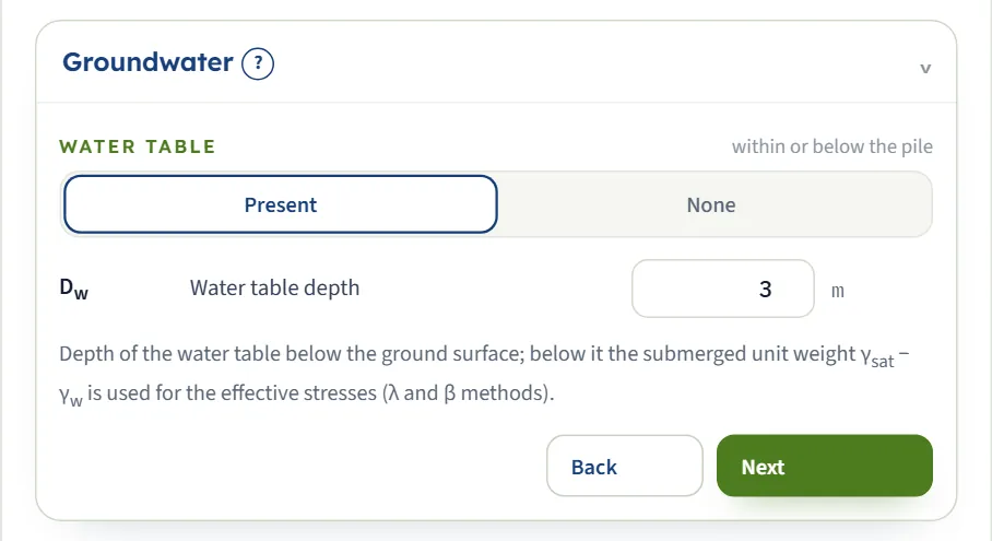
| Choice | Options | Default |
|---|---|---|
| Water table within or below the pile | Present None | Present |
| Field | Symbol | Unit | Default | What to enter |
|---|---|---|---|---|
| Water table depth | Dw | m · ft | 3 | Depth of the water table below the ground surface, 0 or more. Shown when the water table is present. |
Pile
The shape and the installation are choices; the width and the length are numbers. A square pile has Ap = D² and a perimeter of 4D; a circular one Ap = πD²/4 and a perimeter of πD.
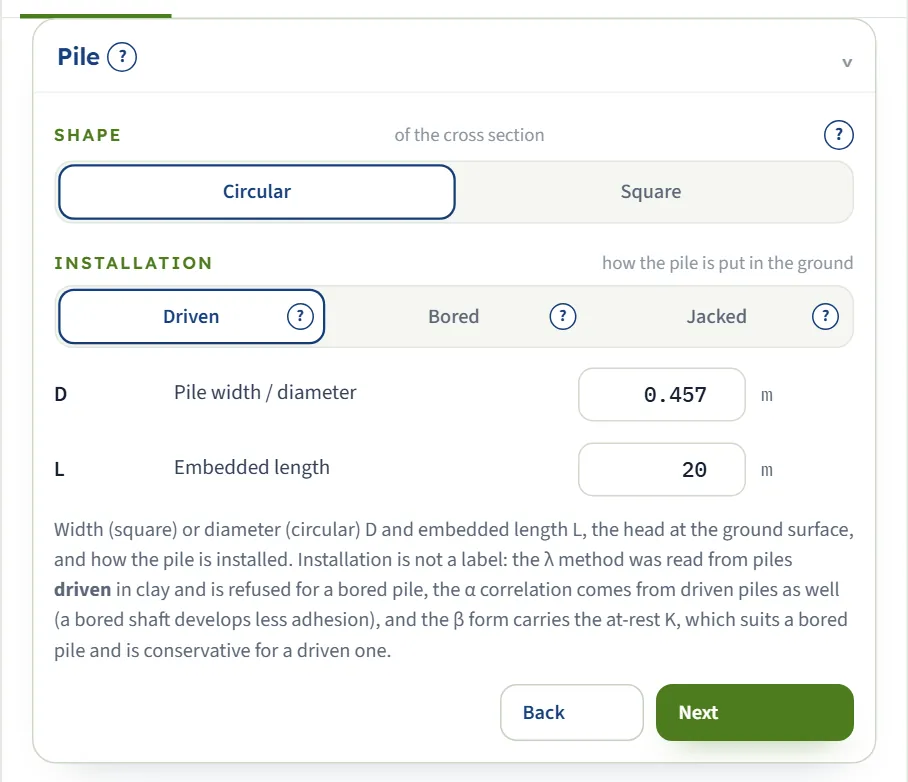
| Choice | Options | Default |
|---|---|---|
| Shape of the cross section | Circular Square | Circular |
| Installation how the pile is put in the ground | Driven Bored Jacked | Driven |
| Field | Symbol | Unit | Default | What to enter |
|---|---|---|---|---|
| Pile width / diameter | D | m · ft | 0.457 | Width of a square pile or diameter of a circular one; it sets the area of the tip and the perimeter of the shaft. |
| Embedded length | L | m · ft | 20 | Embedded length from the ground surface to the tip; the head is at the ground surface. |
Point bearing
Pick the method for the resistance under the tip. Reese & O’Neill is offered for a bored pile only.
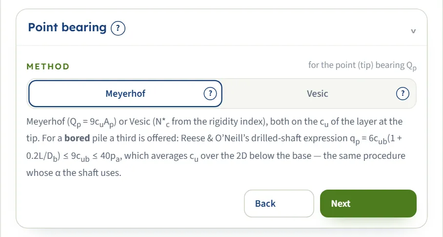
| Choice | Options | Default |
|---|---|---|
| Method for the point (tip) bearing Qp | Meyerhof Vesic Reese & O’Neill | Meyerhof |
Skin friction
Pick the method for the shaft. The α and β methods are worked out layer by layer, with an α or a φ′R for each layer in the boxes below, named after the layer they belong to. The λ method is different in kind: it takes one average over the whole embedded length, so it has no value per layer. The shaft is summed over the embedded length only.
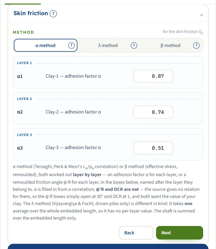
| Choice | Options | Default |
|---|---|---|
| Method for the skin friction Qs | α method λ method β method | α method |
| Field | Symbol | Unit | Default | What to enter |
|---|---|---|---|---|
| Adhesion factor α | α | — | filled in | Adhesion factor of this layer: the share of cu the shaft develops. Filled in from the correlation that belongs to the installation (a driven-pile curve against cu/pa, or 0.55 falling to 0.45 for a bored pile) and editable; the smallest value accepted is 0.05. Shown when skin-friction method is α method. |
| Remoulded drained friction angle | φ′R | ° | 30 | Remoulded drained friction angle of this layer, for the β method. Not filled in from the ground; the box opens at 30° and wants the value of your clay. Shown when skin-friction method is β method. |
Design
One factor of safety on the sum, or a separate factor on each part: Qall = Qp/FSp + Qs/FSs. An applied working load is optional.
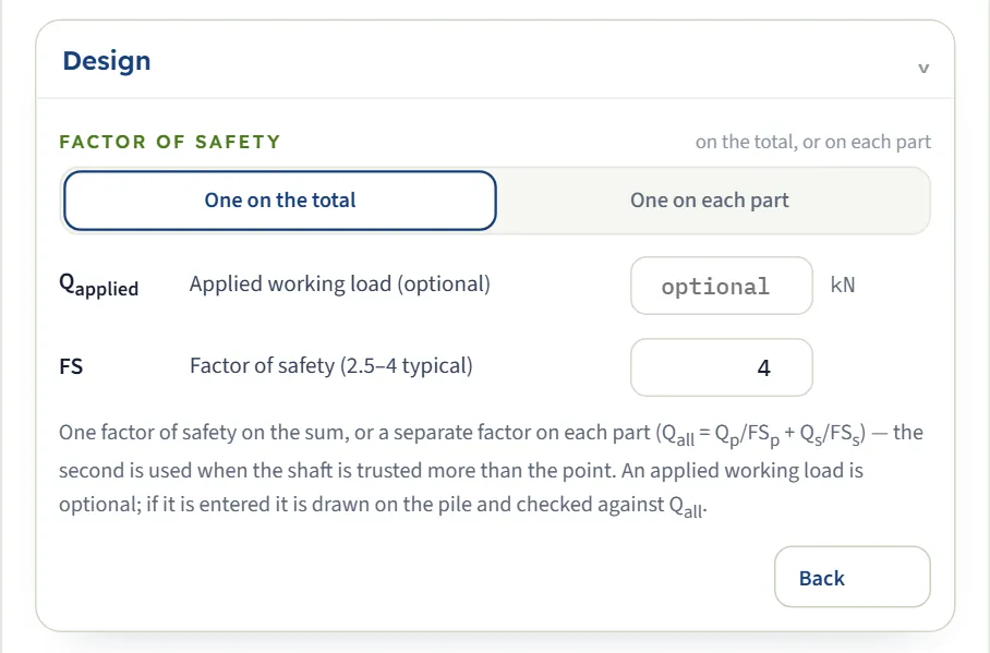
| Choice | Options | Default |
|---|---|---|
| Factor of safety on the total, or on each part | One on the total One on each part | One on the total |
| Field | Symbol | Unit | Default | What to enter |
|---|---|---|---|---|
| Applied working load (optional) | Qapplied | kN · tf · kip | empty | The working load the pile has to carry. Optional: if it is entered it is drawn on the pile and checked against Qall. |
| Factor of safety (2.5–4 typical) | FS | — | 4 | One factor of safety on Qu; the module’s hint is 2.5 to 4. Shown when factor of safety is One on the total. |
| Factor of safety on the point resistance | FSp | — | 4 | Factor of safety on the point resistance (used with one factor on each part). Shown when factor of safety is One on each part. |
| Factor of safety on the skin friction | FSs | — | 2 | Factor of safety on the skin friction. Shown when factor of safety is One on each part. |
Choosing the methods
| Method | Unit resistance qp | Notes |
|---|---|---|
| Meyerhof | qp = 9 cu | cu of the layer at the tip; the strength of the layers above does not enter. The classic deep-foundation value N*c = 9 for saturated clay under undrained loading. |
| Vesic | qp = N*c cu, with N*c from the rigidity index Irr = 347(cu/pa) − 33, limited to 300 | The stiffness of the clay enters through Irr. The correlation starts at about cu = 9.8 kPa; below it the module stops and asks for Meyerhof. |
| Reese & O’Neill (bored piles) | qp = min[6cub(1 + 0.2L/Db), 9cub, 40pa], pa = 100 kPa | cub is the mean cu over the 2D below the base. It follows the same drilled-shaft procedure as the α the shaft uses. For a base wider than 1.91 m the result is reduced by a factor Fr. |
| Method | Unit skin friction | Notes |
|---|---|---|
| α method | f = α cu, layer by layer | An α for each layer, filled in from cu/pa for the installation and editable. Works on total stress: the water table does not change it. |
| λ method (driven piles) | Qs = p L fav, fav = λ(σ̄′ + 2c̄u) | One average over the whole embedded length, with λ read from Vijayvergiya & Focht’s correlation at the pile’s L. The total is then shared among the layers by length. |
| β method | f = β σ′, β = (1 − sin φ′R) tan φ′R √OCR | Effective stress, layer by layer, from the remoulded friction angle and the OCR of each layer. The long-term view: the undrained strength does not enter. |
Which should I pick?
- Start with Meyerhof and the α method. They need only cu and are the module’s defaults.
- Use the λ method for a driven pile when you want the average-condition estimate; it is refused for a bored pile.
- Use the β method when you hold effective-stress parameters (φ′R and OCR) and want the long-term shaft resistance.
- For a bored pile the module fills in the drilled-shaft α and offers Reese & O’Neill for the base.
- Compare. Run the methods one after the other and keep each run with Quick Save…; the what-if table shows how close they come on the example.
Analyze and read the results
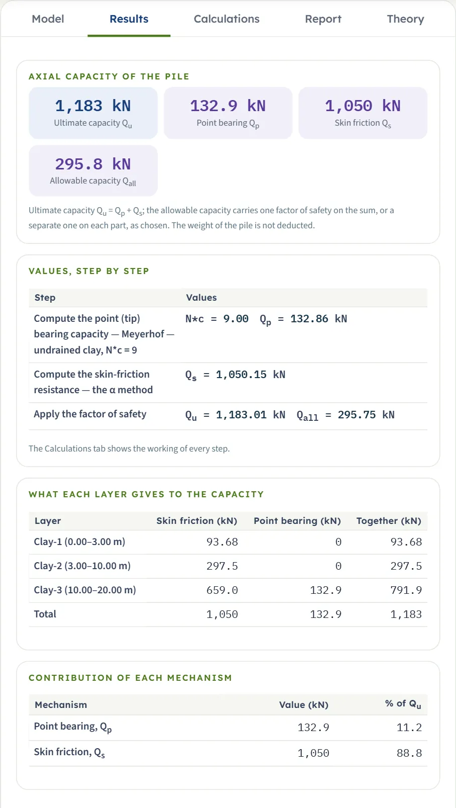
Press Analyze. The bar reports the run, the inputs lock, and the Results tab shows four blocks.
- Axial capacity of the pile. Cards for Qu, Qp, Qs and Qall.
- Values, step by step. The point bearing (N*c, Qp), the shaft (Qs, with λ for that method) and the factor of safety.
- What each layer gives to the capacity. The skin friction, point bearing and total of every layer. With Meyerhof or Vesic the tip layer carries the point bearing; with Reese & O’Neill the table has a row for the base bearing zone, and with the λ method the shaft is shown as one total allocated by length.
- Contribution of each mechanism. The share of the point and of the shaft in Qu.
Checking an applied load
If you enter an applied working load, the Results tab adds the ratio Qapplied/Qall and a verdict in words: PASS when the load is within the allowable capacity, FAIL when it exceeds it. A failing check raises a warning with advice: lengthen or widen the pile, use more piles, or revisit the factors of safety.
The Calculations tab and the report
The Calculations tab starts with Given and what is sought and then follows the method:
- Compute the point (tip) bearing capacity — the method you chose, with cu at the tip, the factor N*c and Qp.
- Compute the skin-friction resistance — the method you chose, with the factors of each layer (α or β) or the averages (λ), and Qs.
- Apply the factor of safety — Qu and Qall.
- Check the applied working load, when one was entered.
The Report tab fills in a cover and saves the same working as a PDF or a Word file: 1 Introduction and scope, 2 Input data, 3 Calculation, 4 Results, then, when the run has notes or warnings about the methods, 5 Assumptions and notes, and finally the Summary and the References. When a run has notes or warnings about the methods, the report adds an Assumptions and notes section after Results; the units line states the conversion constants. The Theory tab explains the method, from why clay is treated as undrained to the three shaft routes compared, the bored-pile procedure and a worked example.
Worked example: the module’s own example
The module opens on this example; Reset to defaults brings it back.
| Layer | Thickness H | cu | γ = γsat | OCR |
|---|---|---|---|---|
| Clay-1 | 3 m | 25 kPa | 16 kN/m³ | 1 |
| Clay-2 | 7 m | 40 kPa | 17 kN/m³ | 1 |
| Clay-3 | 12 m | 90 kPa | 18 kN/m³ | 2 |
Water table at 3 m; circular driven pile, D = 0.457 m, L = 20 m; Meyerhof for the point, the α method for the shaft, one factor of safety FS = 4.
Point bearing
The tip is in Clay-3, so cu = 90 kPa and N*c = 9. The area of the tip is π × 0.457²/4 = 0.1640 m², so Qp = 9 × 90 × 0.16403 = 132.86 kN.
Skin friction
The module fills in α from cu/pa for a driven pile: 0.87, 0.74 and 0.51 for the three layers. The perimeter is π × 0.457 = 1.4357 m and the pile passes through 3 m of Clay-1, 7 m of Clay-2 and 10 m of Clay-3:
| Layer | α | cu (kPa) | Length (m) | α cu perimeter × length (kN) |
|---|---|---|---|---|
| Clay-1 | 0.87 | 25 | 3 | 93.68 |
| Clay-2 | 0.74 | 40 | 7 | 297.48 |
| Clay-3 | 0.51 | 90 | 10 | 658.99 |
| Total Qs | 20 | 1,050.15 |
Capacity
Qu = 132.86 + 1,050.15 = 1,183.01 kN, and with FS = 4, Qall = 295.75 kN. The shaft carries 88.8 % of the capacity and the point 11.2 %: in this example, as usually in clay, the shaft is the larger part, and the Results tab shows which layer gives how much.
How each input changes the answer
Each row changes one thing in the example and runs the module again. The numbers are the results the module gives, in kN.
| Change | Qp | Qs | Qu | Qall | Why |
|---|---|---|---|---|---|
| The default example | 132.9 | 1,050 | 1,183 | 295.8 | The reference |
| Point bearing by Vesic | 168.5 | 1,050 | 1,219 | 304.7 | Irr = 279.3, N*c = 11.41 |
| Skin friction by the λ method | 132.9 | 1,114 | 1,247 | 311.8 | λ = 0.1730 at L = 20 m |
| Skin friction by the β method | 132.9 | 1,058 | 1,191 | 297.8 | β from φ′R = 30° and the OCR of each layer; a note says the at-rest K is on the safe side |
| Bored pile | 132.9 | 928.9 | 1,062 | 265.4 | α = 0.55 in every layer; no friction over the top 1.5 m and the bottom 1D |
| Jacked pile | 132.9 | 1,050 | 1,183 | 295.8 | Same as driven for the α method |
| Jacked pile, λ method | 132.9 | 1,114 | 1,247 | 311.8 | Allowed with a caution: the λ correlation does not cover jacked piles |
| Square section | 169.2 | 1,337 | 1,506 | 376.6 | Larger area and perimeter than the circle of the same D |
| No water table | 132.9 | 1,050 | 1,183 | 295.8 | No change: the α method works on cu alone |
| Water table at 8 m | 132.9 | 1,050 | 1,183 | 295.8 | No change, for the same reason |
| Factor of safety on each part | 132.9 | 1,050 | 1,183 | 558.3 | FSp = 4 and FSs = 2 |
| Pile 14 m long | 132.9 | 654.8 | 787.6 | 196.9 | Less shaft; the point bearing stays |
| Width 0.6 m | 229.0 | 1,379 | 1,608 | 401.9 | Larger tip and perimeter |
| Strength of the tip layer 60 kPa | 88.58 | 925.2 | 1,014 | 253.5 | Lower cu at the tip and in Clay-3 lowers both parts |
| Strength of the first layer 50 kPa | 132.9 | 1,103 | 1,236 | 308.9 | Only the shaft of Clay-1 changes |
Two cases are not in the table because the module does not run them: the λ method for a bored pile, and a pile longer than the layers. It stops and says why (see Messages).
Messages: stops, warnings and notes
The module says in plain words when something prevents the calculation, when a result needs care, and what it assumed.
| Kind | When | Message and what to do |
|---|---|---|
| Stop (brown bar, “Cannot analyse”) | The layers do not reach the pile tip | “the layers must reach the pile tip. They reach 22.00 m, the pile is 24.00 m long.” Add a layer, or thicken the last one. |
| Stop | The λ method for a bored pile | “The λ method was read from piles DRIVEN in clay; a bored pile is outside it.” Use the α method or the β method. |
| Stop | Vesic where cu at the tip is below the start of the correlation | “Vesic’s rigidity index Irr = 347(cu/pa) − 33 has no value at cu = 5.00 kPa; the correlation starts at about 9.80 kPa.” Use Meyerhof for the point. |
| Stop (input error) | A value below the smallest the field accepts | “1 input error: Undrained shear strength (cu,1) must be at least 1 kPa.” Correct the value; for a layer value the row in the table is outlined in red. |
| Warning | The λ method for a jacked pile | “The λ method is for driven piles; this one is jacked.” Read the result as an estimate, or use the α method. |
| Warning | An applied load larger than Qall | “The pile does not carry the applied load — 135.2% of Qall.” Lengthen or widen the pile, use more piles, or revisit the factors of safety. |
| Warning | A bored pile so short that the drilled-shaft exclusions leave no shaft | “The drilled-shaft exclusions leave no shaft to carry friction” (for a bored pile of about L ≤ 1.5 m + D). |
| Note | A bored pile with the α method | The adhesion factors come from the drilled-shaft correlation (α = 0.55 up to cu/pa = 1.5, falling to 0.45 at 2.5), and no shaft resistance is counted over the top 1.5 m or the bottom diameter. |
| Note | A bored pile | The base is taken as clean and the clay beneath it undisturbed; no reduction is applied for the bored construction. |
| Note | The β method for a driven or jacked pile | Computed with the at-rest K = 1 − sin φ′R; a driven pile pushes the clay sideways, so the true K is higher and the result is on the safe side. |
| Note | The β method for a bored pile | The correlation is mainly published for driven piles; for a bored pile the installation and the interface are to be assessed separately. |
| Note | The tip exactly on a layer boundary, or a profile ending just below the tip | The module says which layer carries the base, and that the deepest layer is taken to continue below the described profile. |
The Warnings (or Notes) button on the green bar lists them after a run. They are reflected in the report.
Good practice and common mistakes
- Check that cu is an undrained strength appropriate to the loading, from tests or a reliable correlation. All the α and λ work rests on it.
- Match the installation to the pile. It decides whether the λ method is open and which α is filled in.
- Do not expect the water table to move the α method. It acts on the λ and β methods through the effective stress.
- Enter φ′R and OCR yourself for the β method. They describe your clay, so you enter them: the boxes open at 30° and 1.
- Look at the layer table. In a profile that changes strength with depth the lower layers usually carry most of the shaft, and the table shows which.
- Run more than one method and keep each run with Quick Save….
- Read the notes. They list what the module assumed.
Frequently asked questions
How do I calculate the capacity of a pile in clay?
The ultimate capacity is the point bearing plus the skin friction, Qu = Qp + Qs, and the allowable capacity is Qu divided by a factor of safety. In GeoTerva’s Pile in clay module you describe the clay layers, the pile and the methods, press Analyze, and read Qp, Qs, Qu and Qall with every step of the working.
What is the α method?
The α method gives the unit skin friction of a clay layer as a share of its undrained shear strength, f = α cu. In the module each layer has its own α, filled in from the correlation for the installation, and the shaft is summed over the layers. For a driven pile the example’s layers get 0.87, 0.74 and 0.51; for a bored pile the module uses 0.55 up to cu/pa = 1.5.
What is the λ method?
The λ method works on the whole embedded length at once: Qs = p L λ(σ̄′ + 2c̄u), with the perimeter p, the mean effective stress and the mean undrained strength over the length and λ read from Vijayvergiya & Focht’s correlation at the pile’s length. It applies to driven piles; the module refuses it for a bored pile.
What is the β method?
The β method works on effective stress: f = β σ′ with β = (1 − sin φ′R) tan φ′R √OCR, layer by layer. It needs the remoulded drained friction angle and the OCR of each layer, which you enter. It is the long-term view of the shaft.
Which point-bearing method should I use in clay?
Meyerhof, qp = 9cu, is the default and needs only cu at the tip. Vesic adds the stiffness of the clay through the rigidity index and gave a 27 % larger Qp on the example (N*c = 11.4 against 9). For a bored pile the module also offers Reese & O’Neill’s drilled-shaft expression.
Why does the water table not change my α-method result?
The α method works on the undrained strength cu alone, so the effective stress and the water table do not enter. They do enter the λ and β methods.
Can I use the λ method for a bored pile?
No. It was read from piles driven in clay, so the module stops and asks you to use the α or β method. For a jacked pile it allows the method with a caution.
What does the module do for a bored pile in clay?
It fills in the drilled-shaft α (0.55 up to cu/pa = 1.5, falling to 0.45 at 2.5), with the α method counts no shaft resistance over the top 1.5 m or the bottom diameter, offers Reese & O’Neill for the base, and notes that the base is taken as clean and the clay beneath it undisturbed.
Does the module deduct the weight of the pile?
No. The capacity is the resistance of the ground; the module states under its results that the weight of the pile is not deducted.
How many clay layers can I enter?
Up to eight. Each has its own thickness, cu, unit weights and OCR; the layers must reach at least the pile tip.