

What the module calculates
Pile group takes a group of vertical piles under a rigid cap in layered ground and gives you the load on every pile, the capacity of the group, its settlement and, under a sideways load, the deflection of the cap and the load of every row. Four results answer four questions:
- Which pile takes how much? Every pile of a rigid cap takes its share of the vertical load and of the moments in proportion to its distance from the centroid of the group: P = V/n + B x + C y. The largest and the smallest load, and a pile that is in tension, follow from it.
- What can the group carry? The resistance of one pile is worked out from the ground, layer by layer. The group then acts as individual piles, each layer reduced by the efficiency of its soil, or as one block of soil and piles; the lesser is the capacity: Qg(u) = min(Qind, Qblock) and Qall = Qg(u) / FS.
- How far does it settle? The elastic settlement, by Vesic’s method, plus the consolidation of every clay layer below the level 2L/3 under the 2:1 spread of the load: S = Sg(e) + Sc. You can leave the settlement out.
- How does it move sideways? The cap is rigid, so every pile head has the same deflection Δ. The p–y curves of each row are scaled by the p-multiplier of that row, so the rows carry unequal loads; the module gives Δ, the load and the bending moment of every row.
What you can describe
- A rectangular grid of nx rows of ny piles, or a triangular arrangement at the corners of equilateral triangles; up to 100 rows and 100 piles in a row.
- A ground of up to eight layers, each sand or clay, and an optional water table.
- A circular, hollow circular, square or any other pile section, driven, bored or jacked, with the base of the cap below the ground (zc) or above it (e).
- The loads at the base of the cap: the vertical load V, the lateral load H and the moments My and Mx.
- For every layer its own skin-friction method (K–δ or Coyle & Castello in sand; α, λ or β in clay) and for the base Meyerhof, Vesic, Coyle & Castello or, for a bored pile in clay, Reese & O’Neill.
- Optional limits on the compression and the tension of one pile, the settlement of the group and the deflection of the cap, with a verdict in words.
What belongs to other modules
- The resistance of one pile is worked out here by the methods of Pile on layered soil; nothing about it is typed in. For one pile on its own, with the report of that module, use Pile in sand, Pile in clay or Pile on layered soil.
- The response of one pile to a sideways load, with its deflection, moment and shear diagrams, is the subject of Pile under lateral load. The rows of this module are solved on the same engine.
- The results are loads and movements: the load on every pile and the bending moment along a pile of each row are the loads for the structural design of the pile section, which you make with your own standard.
Before you start: what you need
Have these ready from your ground investigation and your design:
| What | Where it comes from | Notes |
|---|---|---|
| The layout of the piles: rows, piles in a row, spacings | Your design | The spacings are centre to centre. The module flags a spacing under 2.5 pile widths, and a spacing of the rows under 3 widths for the lateral part. |
| The pile: section, width or diameter D, length L, modulus Ep, installation | Your design | Installation decides which methods are open and what the module fills in for the shaft and for the efficiency of a sand layer. |
| The level of the base of the cap | Your design | Below the ground (zc) or above it (e), not both. L is the length of the pile in the ground: measured down from the base of the cap when it is below the ground, from the ground surface when the cap stands above it; the free height e is extra. |
| The ground in layers, each sand or clay | Boring logs | The layers must reach the pile tips. Sand layers need φ′ (20° to 45°), clay layers cu; both need the unit weights. |
| e0, Cc and OCR of the clay layers | Oedometer tests or correlations | Needed only when the settlement is calculated. Cs is optional; empty, it is a fifth of Cc. |
| Water table depth | Piezometers, borings | Optional. |
| The loads at the base of the cap | Your structural analysis | V is the net vertical load with the weight of the cap included. A lateral load at a height h above the base of the cap gives a moment M = H h. |
| Es and νs of the soil below the base | Tests or correlations | Needed for the elastic settlement. Leave Es empty to leave the elastic part out. |
| Factor of safety; allowable loads and movements | Your design basis | The factor of safety is on the capacity of the group and of one pile. The four limits are optional. |
Quick start in ten steps
- Open the module and choose the units
Open Pile group from the Piles family. Pick SI · kN, SI · tf or US in the header; you can change it at any time. Open Pile group.
- Describe the group
In Group, choose the Rectangular grid or the Triangular (equilateral) arrangement, then give the number of rows nx, the piles in a row ny and the spacings.
- Describe the pile and the cap
In Pile, choose the section and the installation (Driven, Bored or Jacked), then enter D, Ep, the embedded length L and the level of the base of the cap.
- Describe the soil layers and the water
In Soil layers, fill in the New layer form (sand or clay, thickness, unit weights, φ′ or cu) and press + Add layer; repeat from the ground surface down. The layers must reach the pile tips. In Groundwater choose Present with its depth, or None.
- Enter the loads
In Loading, enter V, H, My and Mx at the base of the cap.
- Choose the methods
In Point bearing pick the method for the base. In Skin friction every layer shows the methods of its own soil; the coefficients are filled in and can be typed over.
- Decide on the settlement
In Settlement choose Calculated and give Es, νs and ξ, or Not calculated to leave the settlement out.
- Check the lateral group effect
In Lateral group effect choose whether the pile heads are held against rotation or free, whether the loading is static or cyclic, and whether the load acts in one direction or reverses. The p–y constants and the p-multipliers are filled in from the layers and the spacing.
- Set the design values
In Design, enter the factor of safety and, if you want a verdict, the allowable compression and tension of one pile, the allowable settlement and the allowable deflection of the cap.
- Press Analyze and read the answer
Press Analyze. The Results tab gives the loads, the capacity, the settlement and the lateral response; the five views of the drawing carry the numbers; the Calculations tab shows every step; the Report tab saves a PDF or a Word file.
The screen: five views of the group
The layout is the one every GeoTerva module shares, described in the workspace guide. For this module the drawing has five views, chosen with the buttons above it. Changing the unit system redraws the views in the new units. Plan and Section follow your inputs as you type; Capacity, Settlement and Lateral show results and are available after Analyze.
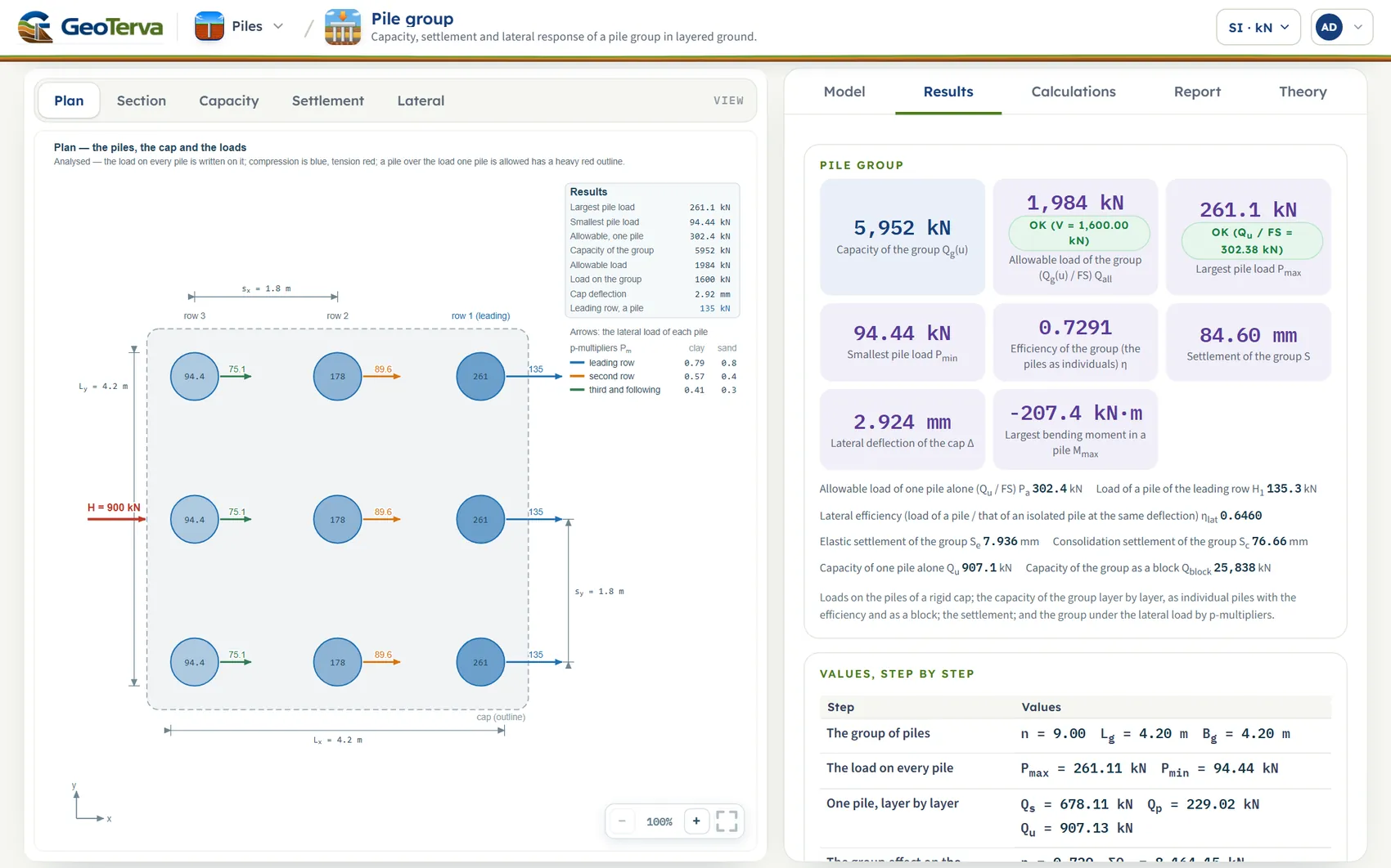
- Plan. The piles, the cap and the loads; after Analyze the load on every pile.
- Section. The piles in the ground, the layers and the spread of the load.
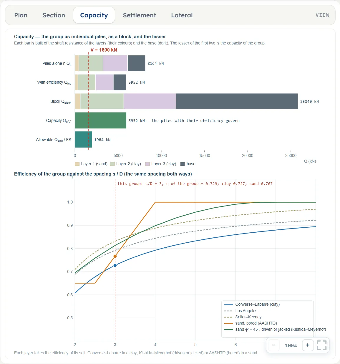
- Capacity. The capacity of the group as individuals, as a block, and the efficiency against the spacing.
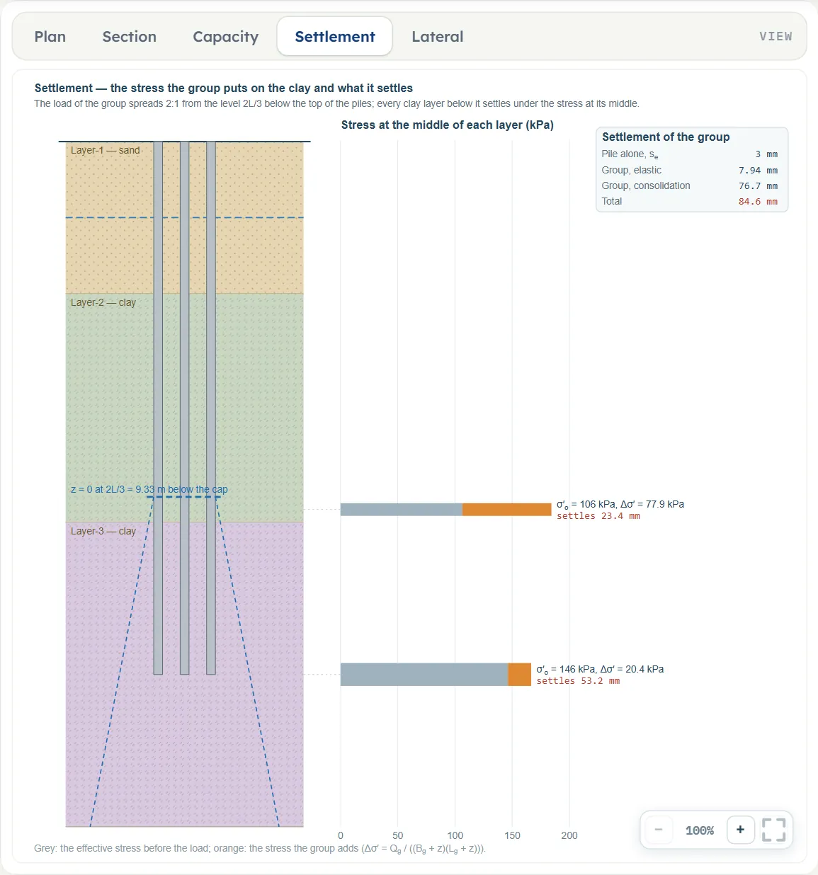
- Settlement. The stress the group puts on each clay layer and what each settles.
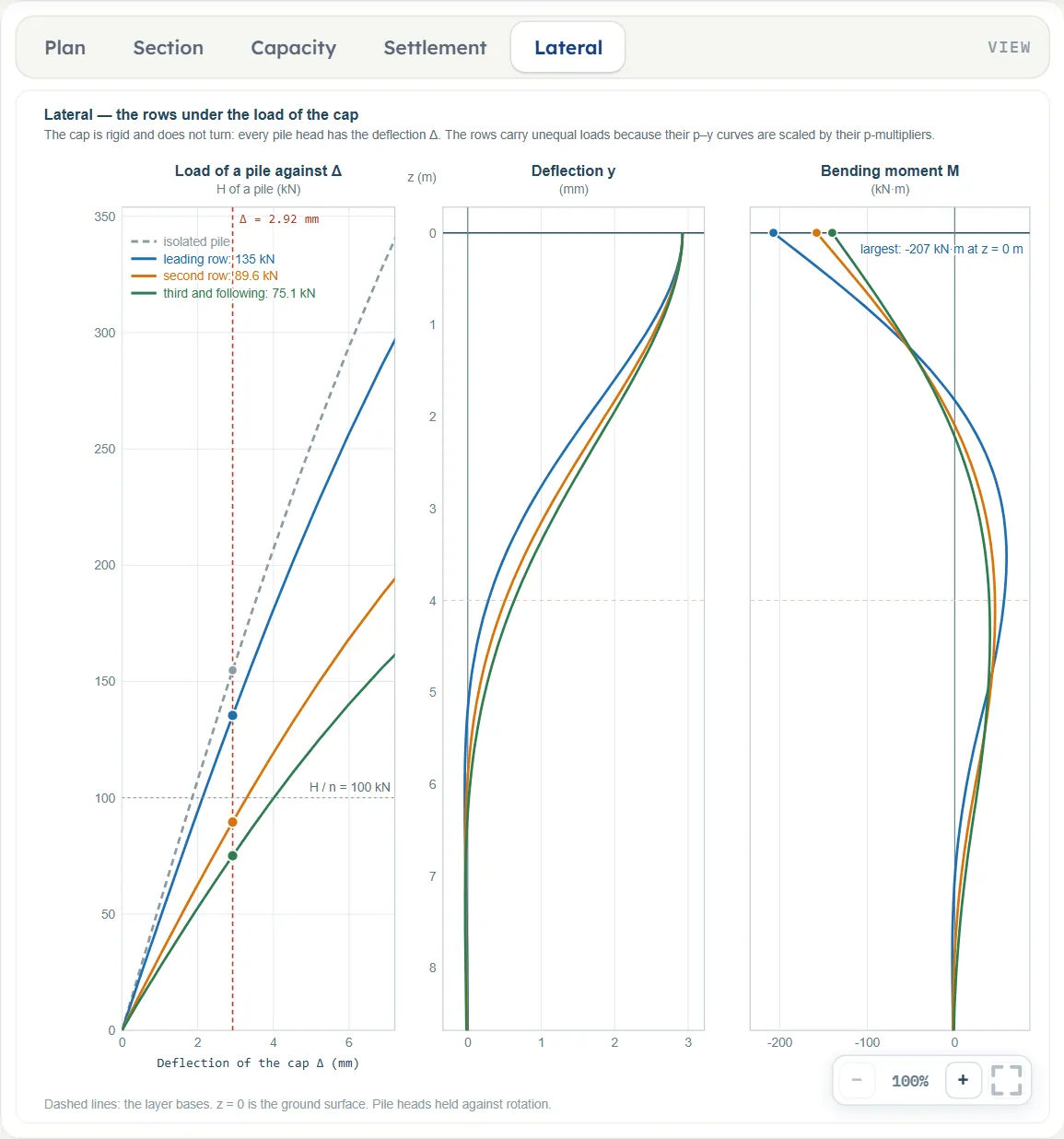
- Lateral. The rows under the load of the cap: load, deflection and bending moment.
- Results box. On the drawing: the main numbers of the run, in the unit system of the page.
- Tabs. Model, Results, Calculations, Report and Theory.
- Cards. On the Results tab: the capacity, the loads on the piles, the settlement and the lateral response, each with its verdict where a limit applies.
Plan
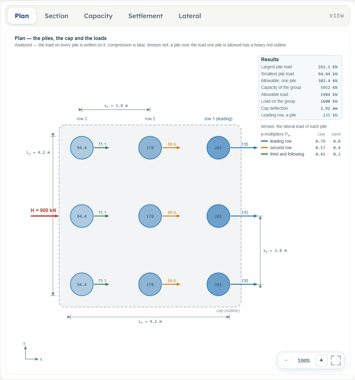
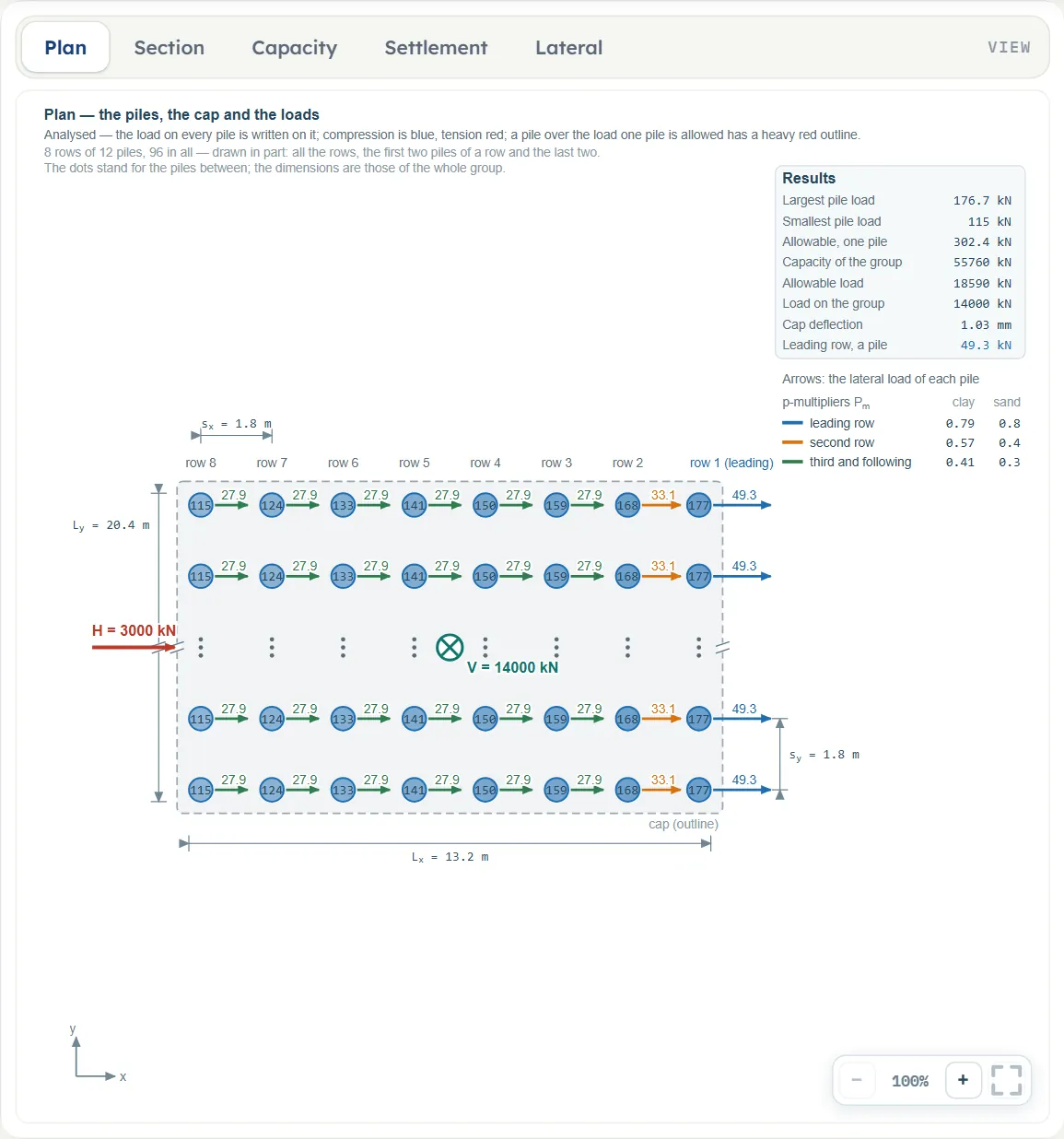
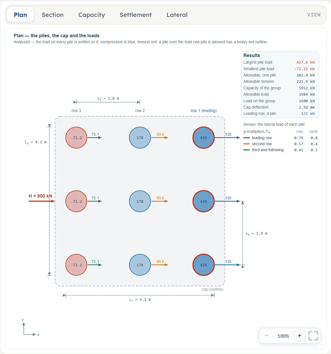
The piles in plan, with the loads on the cap and the dimensions of the group. The rows are numbered from the front: row 1, the leading row, is the one the lateral load pushes towards, and the rows behind it stand in its shadow. After Analyze the load on every pile is written on it: compression is blue, tension red, and a pile over the load one pile alone is allowed has a heavy red outline. An arrow on each pile gives its share of the lateral load, and a small table lists the p-multipliers of the three kinds of row.
A group of more than eight rows, or of more than eight piles in a row, is drawn in part: the first two rows and the last three rows, and the first two piles and the last two piles of a row, with dots between them, as a matrix is written. The dimensions on the drawing keep the real values.
Section
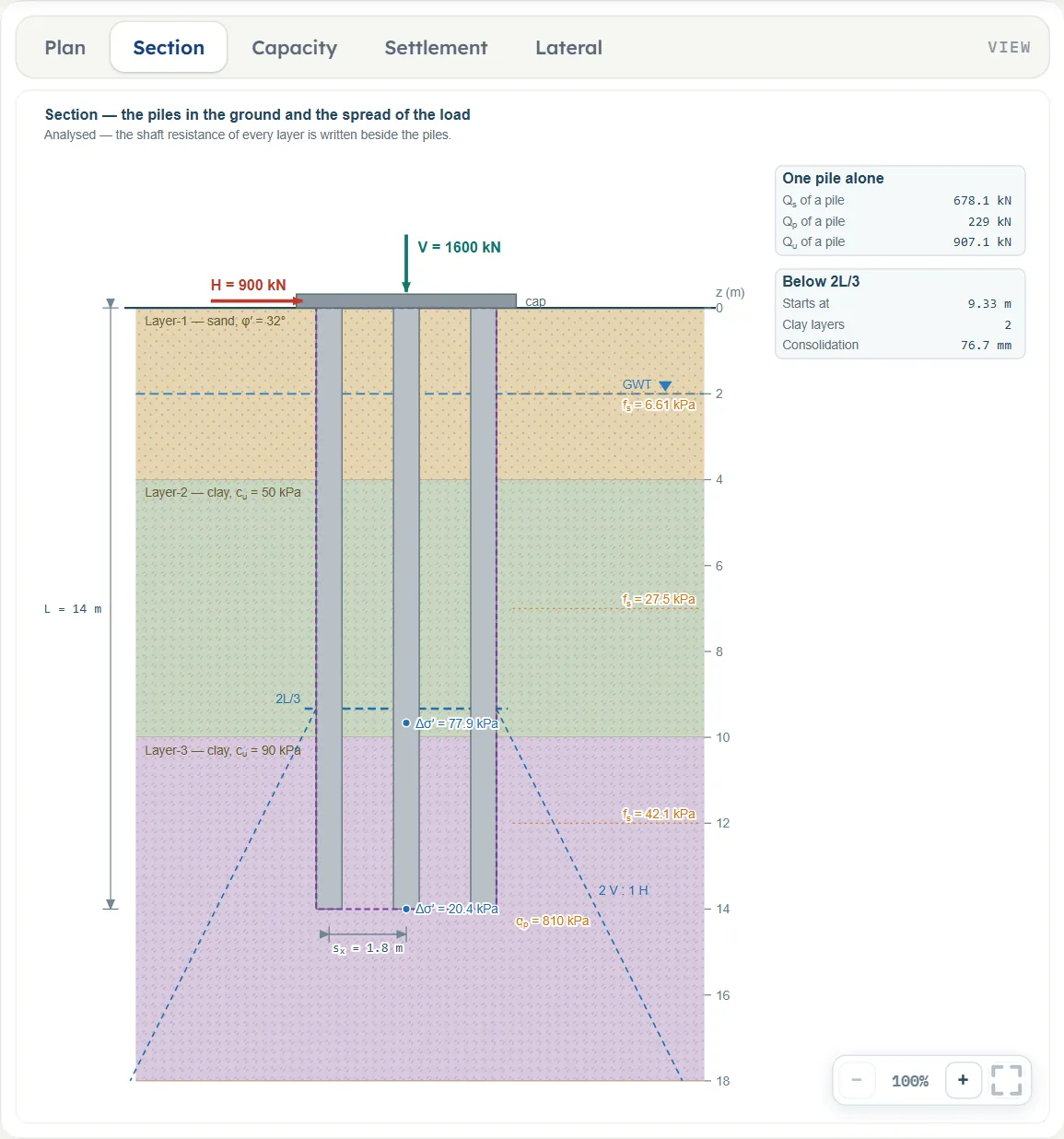
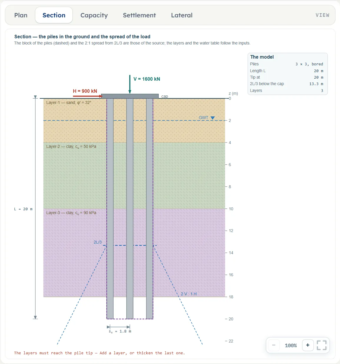
The piles in the ground: the layers with their soil, the water table, the cap, the level 2L/3 below the top of the piles and the 2:1 spread of the load below it. After Analyze each layer carries the unit shaft resistance fs, the base the unit resistance qp, and the middle of each clay layer below 2L/3 the stress Δσ′ the group adds there. Two boxes give the resistance of one pile alone (Qs, Qp, Qu) and the start of the spread.
Capacity
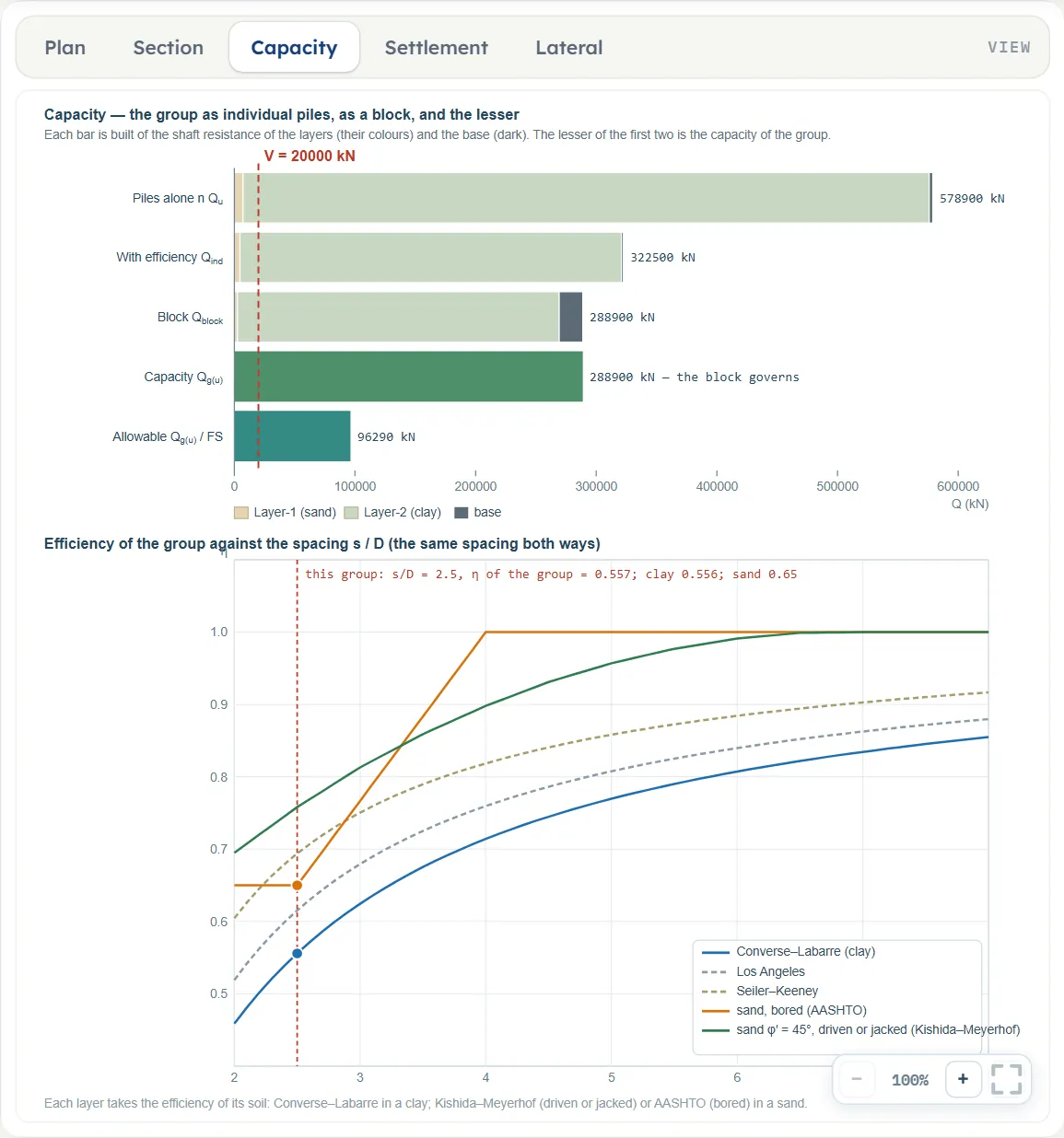
Five bars built of the layers they take their resistance from, with the base in a dark colour: the piles alone (n Qu), the piles with their efficiency (Qind), the block (Qblock), the capacity Qg(u) (the lesser of the two) and the allowable load Qall. A dashed line marks the vertical load V. Below, the efficiency against the spacing s/D: the equation of Converse and Labarre for clay, the chart of Kishida and Meyerhof and the AASHTO rule for sand, and two other equations drawn for comparison, with a vertical line at the spacing of your group.
Settlement
The ground on the left with the group and the 2:1 spread; on the right, for every clay layer below 2L/3, a bar at the middle of the layer: grey for the effective stress before the load, orange for the stress Δσ′ the group adds, and the settlement of the layer written beside it. A box gives the elastic part, the consolidation and the total. Nothing is drawn when the settlement is left out.
Lateral
The rows under the load of the cap. Left: the load of a pile against the deflection Δ for the leading row, the second row, the third and the rows behind it, and an isolated pile, with the deflection of the cap marked. Middle and right: the deflection and the bending moment along a pile of each kind of row, with the largest moment marked.
Entering the model, section by section
The Model tab has ten sections after Model data. Each opens when you click its title; Next and Back at the foot walk you through them. A (?) beside a title or a method opens a help window with a drawing and the formula for that part. The tables list the fields with their symbol, the unit in each unit system and their default. Where a unit is shown twice or three times, such as m · ft, the units are those of SI · kN, SI · tf and US in turn, and equal ones are merged. The defaults are those of SI · kN: in US the spacing of 1.8 m shows as 5.90551 ft and V = 1600 kN as 359.694 kip. A field marked “filled in” carries a value the module works out from your other inputs; you can type over it, and emptying the box gives the module’s value back. The fields of a layer are listed once, for layer 1.
Group
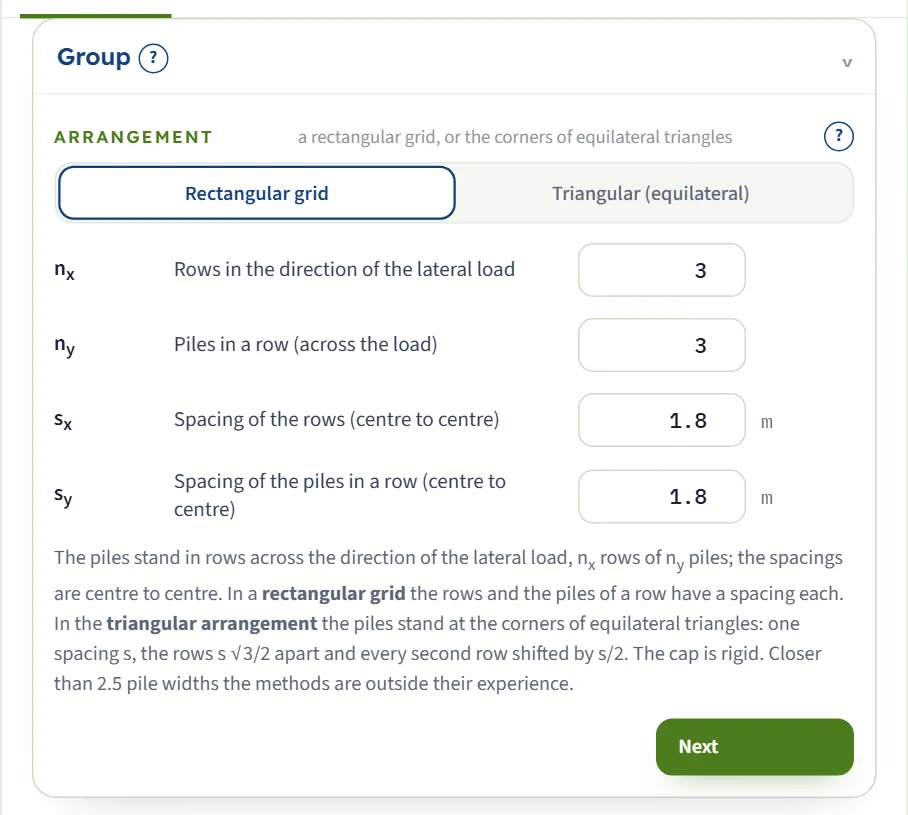
The arrangement, the number of rows and of piles in a row, and the spacings. The piles stand in rows across the direction of the lateral load, nx rows of ny piles, under a rigid cap. In the rectangular grid the rows and the piles of a row each have a spacing. In the triangular arrangement one spacing s serves all: the piles of a row are s apart, the rows s √3/2 apart and every second row is shifted by s/2. The module flags a spacing under 2.5 pile widths.
| Choice | Options | Default |
|---|---|---|
| Arrangement a rectangular grid, or the corners of equilateral triangles | Rectangular grid Triangular (equilateral) | Rectangular grid |
| Field | Symbol | Unit | Default | What to enter |
|---|---|---|---|---|
| Rows in the direction of the lateral load | nx | — | 3 | Number of rows, one behind the other along the lateral load. A whole number, 1 to 100. Row 1 is the leading row. |
| Piles in a row (across the load) | ny | — | 3 | Piles in each row, side by side across the load. A whole number, 1 to 100. |
| Spacing of the rows (centre to centre) | sx | m · ft | 1.8 | Spacing of the rows, centre to centre, along the lateral load. It sets the p-multipliers. It must be larger than D. Shown when arrangement of the piles is Rectangular grid. |
| Spacing of the piles in a row (centre to centre) | sy | m · ft | 1.8 | Spacing of the piles in a row, centre to centre. It must be larger than D. Shown when arrangement of the piles is Rectangular grid. |
| Spacing of the piles (centre to centre) | s | m · ft | 1.8 | One spacing for the triangular arrangement: the piles of a row are s apart, the rows s √3/2 apart, and every second row is shifted by s/2. It must be larger than D. Shown when arrangement of the piles is Triangular (equilateral). |
Pile
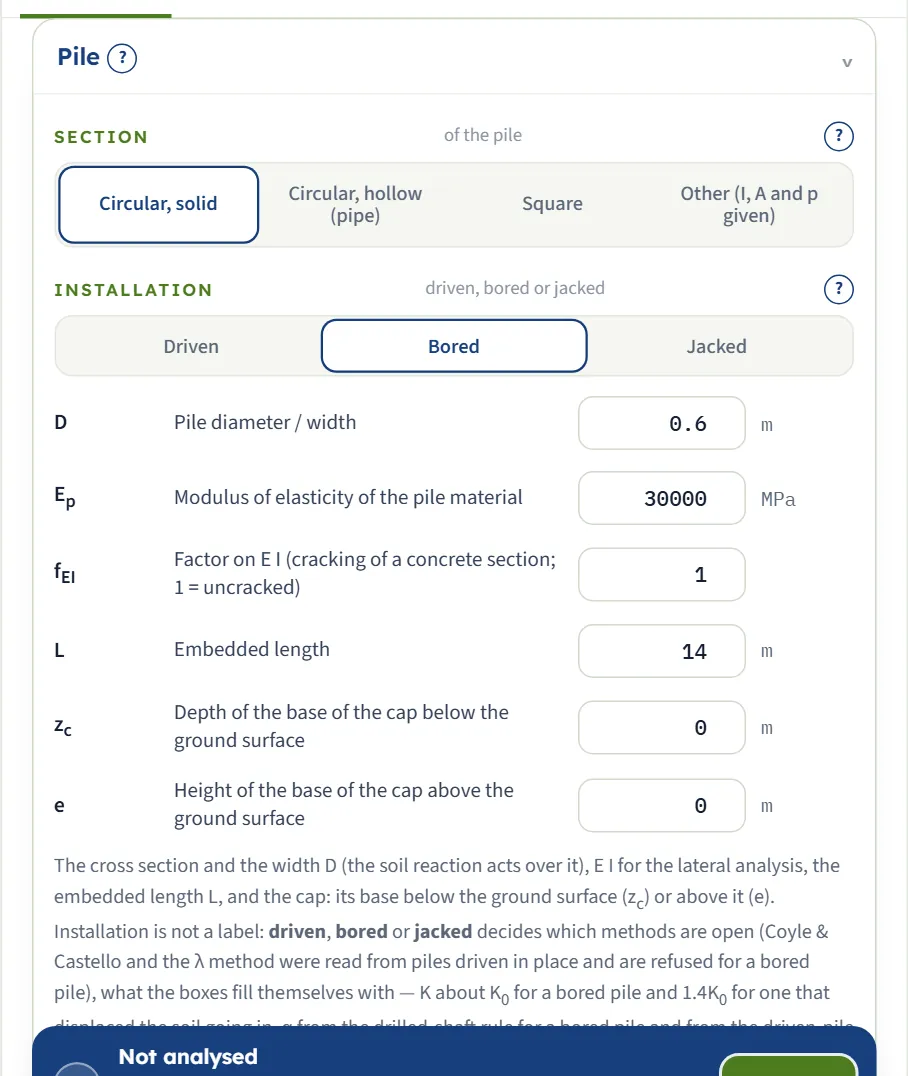
The section, the installation, the size and stiffness of the pile and the level of the base of the cap. The section gives the area of the base, the perimeter of the shaft and, with Ep and fEI, the bending stiffness E I of the lateral analysis; for Other (I, A and p given) you enter I, A and p yourself. For a hollow pipe the base uses the full outer circle, so a pipe pile gives the same capacity as a solid pile of the same D (5,952 kN for the group of the example); the wall thickness t enters the stiffness and the elastic shortening.
| Choice | Options | Default |
|---|---|---|
| Section of the pile | Circular, solid Circular, hollow (pipe) Square Other (I, A and p given) | Circular, solid |
| Installation driven, bored or jacked | Driven Bored Jacked | Bored |
| Field | Symbol | Unit | Default | What to enter |
|---|---|---|---|---|
| Pile diameter / width | D | m · ft | 0.6 | Diameter of a circular pile or width of a square one. For a section given by I, A and p it is still the width the soil reaction acts over. |
| Wall thickness of the pipe | t | m · ft | 0.02 | Wall thickness of the pipe, between 0 and D/2. Shown when section is Circular, hollow (pipe). |
| Second moment of area about the axis of bending | I | cm⁴ · in⁴ | 636170 | Second moment of area about the axis of bending. Shown when section is Other (I, A and p given). |
| Cross-section area (also the area of the base) | A | cm² · in² | 2827 | Area of the section; also the area of the base. Shown when section is Other (I, A and p given). |
| Perimeter of the pile | p | m · ft | 1.885 | Perimeter of the section. Shown when section is Other (I, A and p given). |
| Modulus of elasticity of the pile material | Ep | MPa · kg/cm² · ksi | 30000 | About 30 000 MPa for a concrete pile, 200 000 MPa for steel. |
| Factor on E I (cracking of a concrete section; 1 = uncracked) | fEI | — | 1 | Factor on E I for the lateral analysis: 1 for an uncracked section; 0.5 to 0.8 is common practice for a cracked concrete section. Accepted from 0.05 to 1.5. |
| Embedded length | L | m · ft | 14 | Length of the pile in the ground, measured down from the base of the cap when it is below the ground (zc), or from the ground surface when the cap stands above it (e); the free height e is extra. |
| Depth of the base of the cap below the ground surface | zc | m · ft | 0 | Depth of the base of the cap below the ground surface. The soil above it counts in the stresses of the axial analysis; the lateral analysis starts at the base of the cap. |
| Height of the base of the cap above the ground surface | e | m · ft | 0 | Height of the base of the cap above the ground surface; the piles stand free over this height. Enter zc or e, not both. |
Soil layers
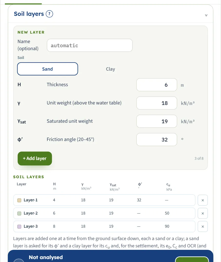
Up to eight layers, entered from the ground surface down, each Sand or Clay. A sand layer is asked for φ′, a clay layer for cu and, when the settlement is calculated, for e0, Cc, OCR and optionally Cs. The layers must reach the pile tips; the module takes the deepest layer to continue below the profile when it ends within 2D of the tips, and says so. The New layer form opens at H = 6 m; the table below lists the three layers of the example (4, 6 and 8 m), and the field table shows the defaults of layer 1 (H = 4 m, cu = 40 kPa), while the clays of the example have cu = 50 and 90 kPa. Everything that follows is worked out layer by layer from what you enter here.
- Fill in the New layer form and press + Add layer; the layer joins the Soil layers table and the counter (“3 of 8”) moves on.
- Click a row to edit a layer; the cross at the end of a row removes it.
| Field | Symbol | Unit | Default | What to enter |
|---|---|---|---|---|
| Name (optional) | — | — | empty | A name for the layer, for the drawings and the report. Left empty, the layers are called Layer-1, Layer-2 and so on. |
| Thickness | H | m · ft | 4 | Thickness of the layer; the smallest value accepted is 0.1 m. The layers together must reach the pile tips. |
| Unit weight (above the water table) | γ | kN/m³ · t/m³ · pcf | 18 | Unit weight above the water table. |
| Saturated unit weight | γsat | kN/m³ · t/m³ · pcf | 19 | Unit weight below the water table; it must be above the unit weight of water. Used only when a water table is present. Shown when water table is Present. |
| Friction angle (20–45°) | φ′ | ° | 32 | Effective friction angle of a sand layer, 20° to 45°: the base resistance of Meyerhof is tabulated for this range, and outside it the module stops. Shown when the layer is sand. |
| Undrained shear strength | cu | kPa · kg/cm² · psf | 40 | Undrained shear strength of a clay layer. Shown when the layer is clay. |
| Overconsolidation ratio | OCR | — | 1 | 1 is a normally consolidated clay, the safe side for the settlement (it settles most). Used by the consolidation settlement and by the β method. Shown when the layer is clay. |
| Initial void ratio | e0 | — | 0.9 | Initial void ratio of the clay layer. Shown when the layer is clay and settlement of the group is Calculated. |
| Compression index | Cc | — | 0.28 | Compression index of the clay layer. Shown when the layer is clay and settlement of the group is Calculated. |
| Recompression index (optional) | Cs | — | empty | Recompression index, used where the stress stays below the preconsolidation pressure. Left empty it is a fifth of Cc. Shown when the layer is clay and settlement of the group is Calculated. |
Groundwater
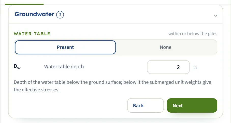
Choose whether there is a water table and, if there is, its depth. Below it the effective stresses use the unit weight γsat − γw of the layer, with γw = 9.81 kN/m³.
| Choice | Options | Default |
|---|---|---|
| Water table within or below the piles | Present None | Present |
| Field | Symbol | Unit | Default | What to enter |
|---|---|---|---|---|
| Water table depth | Dw | m · ft | 2 | Depth of the water table below the ground surface, 0 or more. Below it the effective stresses use the submerged unit weights. Shown when water table is Present. |
Loading
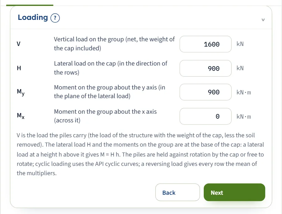
The loads act at the base of the cap. V is the load the piles carry: the load of the structure with the weight of the cap, less the weight of any soil removed. The lateral load H acts along x, the direction of the rows, and meets the rows one after another. A lateral load at a height h above the base of the cap is entered as H and as the moment My = H h.
| Field | Symbol | Unit | Default | What to enter |
|---|---|---|---|---|
| Vertical load on the group (net, the weight of the cap included) | V | kN · tf · kip | 1600 | Net vertical load on the group, in compression, with the weight of the cap included and the weight of the soil removed deducted. |
| Lateral load on the cap (in the direction of the rows) | H | kN · tf · kip | 900 | Lateral load on the cap, along x, the direction of the rows, at the base of the cap. |
| Moment on the group about the y axis (in the plane of the lateral load) | My | kN·m · tf·m · kip·ft | 900 | Moment on the group about the y axis, in the plane of the lateral load. Positive: more compression on the side the lateral load pushes towards. A lateral load at a height h above the base of the cap gives H h. |
| Moment on the group about the x axis (across it) | Mx | kN·m · tf·m · kip·ft | 0 | Moment about the x axis, across the lateral load. Positive: more compression on the +y side. |
Point bearing
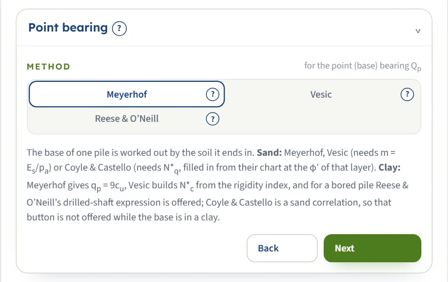
Pick the method for the resistance under the tip. The base of a pile is worked out by the soil it ends in: in a sand by Meyerhof, Vesic or Coyle & Castello; in a clay by Meyerhof (qp = 9 cu), by Vesic (which builds N*c from the rigidity index) or, for a bored pile, by the drilled-shaft expression of Reese & O’Neill. Coyle & Castello’s charts are a sand correlation, so that button is not offered while the base is in a clay, and Reese & O’Neill is offered only for a bored pile whose base is in a clay.
| Choice | Options | Default |
|---|---|---|
| Method for the point (base) bearing Qp | Meyerhof Vesic Coyle & Castello Reese & O’Neill | Meyerhof |
| Field | Symbol | Unit | Default | What to enter |
|---|---|---|---|---|
| Es/pa (only used if the base is on a sand and Vesic is selected) | m | — | 250 | Stiffness ratio Es/pa of the sand at the base, for Vesic’s method. The smallest value accepted is 50. Shown when point-bearing method is Vesic. |
| Coyle & Castello N*q — chart default for this pile, editable | N*q(CC) | — | filled in | Read from the Coyle & Castello chart for this pile’s L/D and the φ′ of the layer the base stands in, and kept up to date. Type over it to use your own reading. Shown when point-bearing method is Coyle & Castello. |
Skin friction
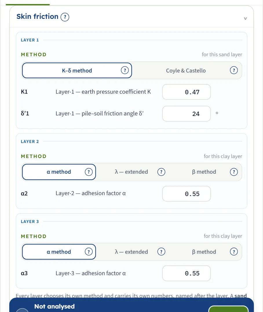
Every layer chooses its own method and carries its own numbers, named after the layer. The methods are those of Pile on layered soil, and each shows only the boxes it needs:
| Soil | Methods | Boxes |
|---|---|---|
| Sand layer | K–δ method; Coyle & Castello | K and δ′ for the K–δ method; KCC for Coyle & Castello. All are filled in and can be typed over. |
| Clay layer | α method; λ — extended; β method | α for the α method (filled in); nothing for the λ method; φ′R for the β method (typed by you, with the OCR of the layer). |
| Field | Symbol | Unit | Default | What to enter |
|---|---|---|---|---|
| Earth pressure coefficient K | K | — | filled in | Earth pressure coefficient on the shaft in this layer. Filled in as K0 = 1 − sin φ′ for a bored pile and 1.4 K0 for a driven or jacked one. The smallest value accepted is 0.2. Shown when the layer is sand and the skin-friction method of the layer is K–δ method. |
| Pile–soil friction angle δ′ | δ′ | ° | filled in | Friction angle between the pile and the sand in this layer. Filled in as 0.75 φ′. Shown when the layer is sand and the skin-friction method of the layer is K–δ method. |
| Coyle & Castello K | KCC | — | filled in | Coyle & Castello’s coefficient for this layer, read from their chart at the layer’s φ′ and the pile’s L/D; the interface friction is 0.8 φ′. Editable. Shown when the layer is sand and the skin-friction method of the layer is Coyle & Castello. |
| Adhesion factor α | α | — | filled in | Adhesion factor on cu. Filled in from the drilled-shaft rule of O’Neill & Reese for a bored pile and from the driven-pile curve otherwise (0.55 in the example). Between 0.05 and 1. Shown when the layer is clay and the skin-friction method of the layer is α method. |
| Remoulded drained friction angle | φ′R | ° | 30 | Remoulded drained friction angle of the clay, for the β method. It is not filled in: no correlation is given for it, so the box opens at 30° and wants the value of your clay. Shown when the layer is clay and the skin-friction method of the layer is β method. |
Settlement
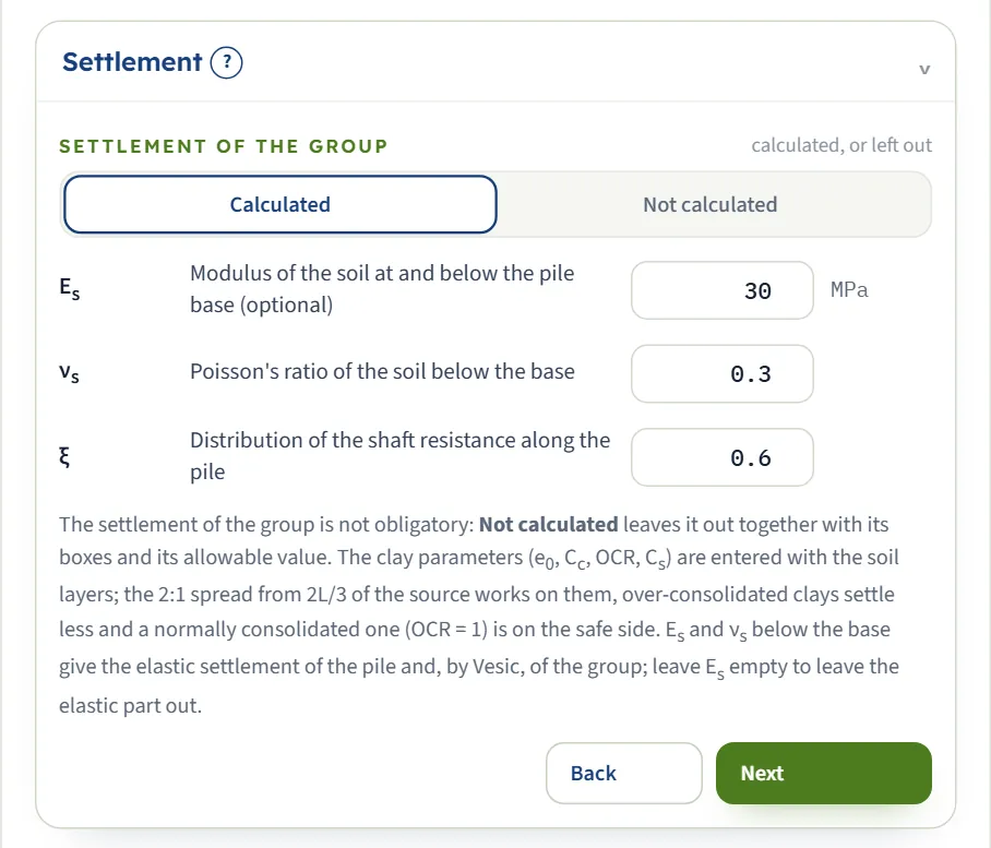
The settlement of the group is not obligatory. Not calculated leaves it out together with its boxes and its allowable value, and the Settlement view draws nothing; the loads, the capacity and the lateral response are worked out either way. With Calculated, the clay parameters entered with the soil layers drive the consolidation, and Es, νs and ξ below the base give the elastic settlement of a pile and, by Vesic’s factor, of the group; leave Es empty to leave the elastic part out.
| Choice | Options | Default |
|---|---|---|
| Settlement of the group calculated, or left out | Calculated Not calculated | Calculated |
| Field | Symbol | Unit | Default | What to enter |
|---|---|---|---|---|
| Modulus of the soil at and below the pile base (optional) | Es | MPa · kg/cm² · ksf | 30 | Modulus of the soil at and below the pile base, for the elastic settlement of a pile and, with it, of the group. Leave it empty to leave the elastic part out. Shown when settlement of the group is Calculated. |
| Poisson's ratio of the soil below the base | νs | — | 0.3 | Poisson’s ratio of the soil below the base, 0 to 0.5. Shown when settlement of the group is Calculated. |
| Distribution of the shaft resistance along the pile | ξ | — | 0.6 | Distribution of the shaft resistance along the pile, for the shortening of the pile: 0.5 for a uniform one, 0.67 for one increasing with depth. The module accepts 0.5 to 0.67. Shown when settlement of the group is Calculated. |
Lateral group effect
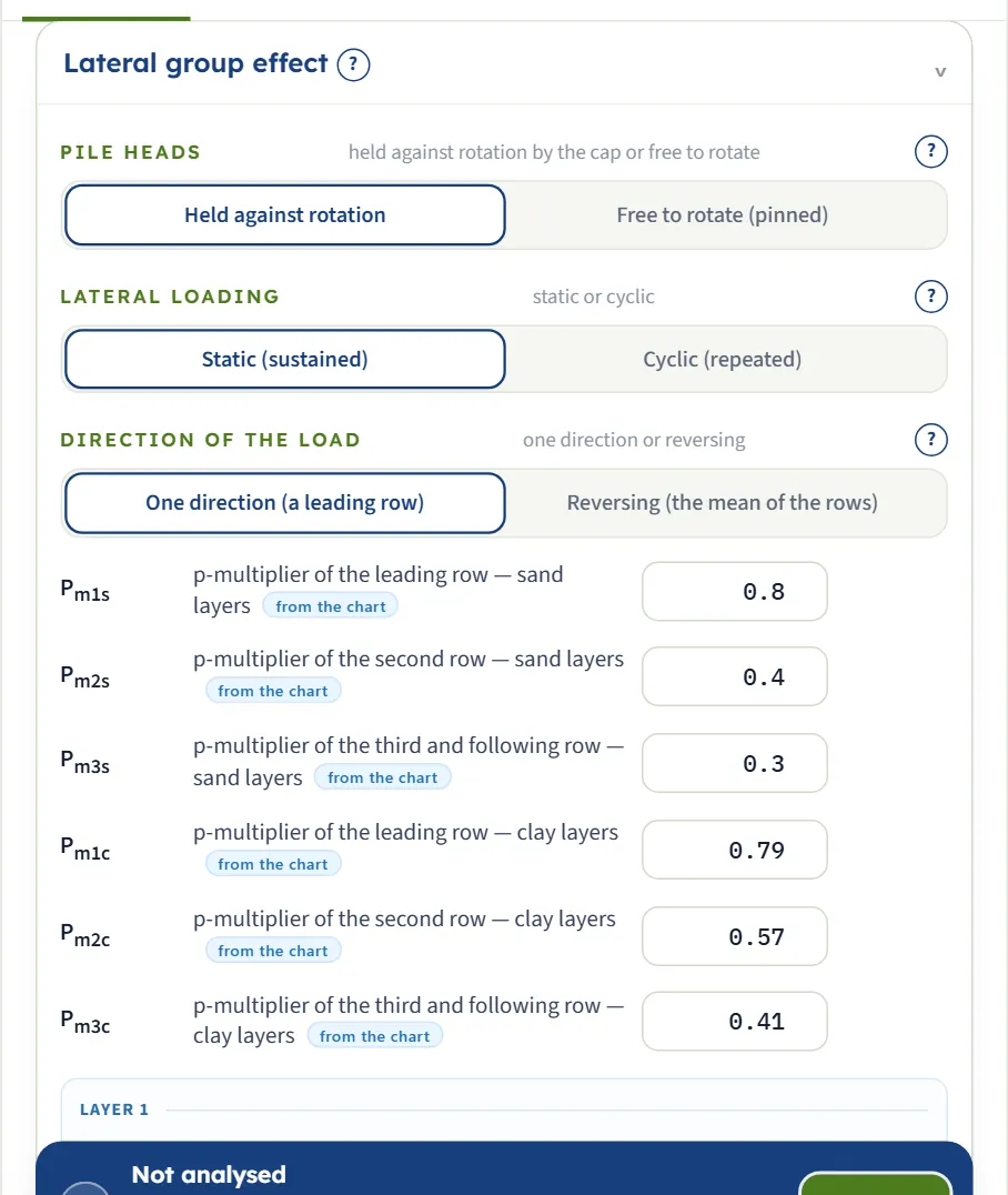
How the pile heads are held, how the load acts, and the constants of the p–y curves. Held against rotation is a pile head fixed in the cap; Free to rotate (pinned) a pinned one. Static (sustained) loading uses the p–y curves as they stand; Cyclic (repeated) the cyclic curves of API RP 2A. One direction (a leading row) gives each row its own multiplier; Reversing (the mean of the rows) gives every row the mean of the multipliers. The constants of the p–y curves of each layer and the six p-multipliers are filled in; see Choosing the methods for what they are.
| Choice | Options | Default |
|---|---|---|
| Pile heads held against rotation by the cap or free to rotate | Held against rotation Free to rotate (pinned) | Held against rotation |
| Lateral loading static or cyclic | Static (sustained) Cyclic (repeated) | Static (sustained) |
| Direction of the load one direction or reversing | One direction (a leading row) Reversing (the mean of the rows) | One direction (a leading row) |
| Field | Symbol | Unit | Default | What to enter |
|---|---|---|---|---|
| P-multiplier of the leading row — sand layers | Pm1s | — | filled in | Factor on the p–y curves of the sand layers for a pile of the leading row. Filled in from the spacing of the rows (AASHTO LRFD); type over it to use your own. |
| P-multiplier of the second row — sand layers | Pm2s | — | filled in | The same for a pile of the second row. |
| P-multiplier of the third and following row — sand layers | Pm3s | — | filled in | The same for a pile of the third row and of every row behind it. |
| P-multiplier of the leading row — clay layers | Pm1c | — | filled in | Factor on the p–y curves of the clay layers for a pile of the leading row. Filled in from the spacing of the rows (Rollins et al., 2006); type over it to use your own. |
| P-multiplier of the second row — clay layers | Pm2c | — | filled in | The same for a pile of the second row. |
| P-multiplier of the third and following row — clay layers | Pm3c | — | filled in | The same for a pile of the third row and of every row behind it. |
| Field | Symbol | Unit | Default | What to enter |
|---|---|---|---|---|
| Initial modulus k of the p–y curve | k | MN/m³ · t/m³ · pci | filled in | Initial modulus k of the sand p–y curve: the slope at the origin is k z. Filled in from φ′ and the water; type over it to use your own. Shown when the layer is sand. |
| Strain ε50 at half the strength | ε50 | — | filled in | Strain at half the strength, for the clay p–y curve: y50 = 2.5 ε50 D. Filled in from cu (0.020 soft, 0.010 medium, 0.005 stiff). Shown when the layer is clay. |
| Matlock J | J | — | filled in | Matlock’s constant for the near-surface wedge of a clay: 0.5 for a soft clay, 0.25 for a medium to stiff one. Filled in from cu. Shown when the layer is clay. |
Design
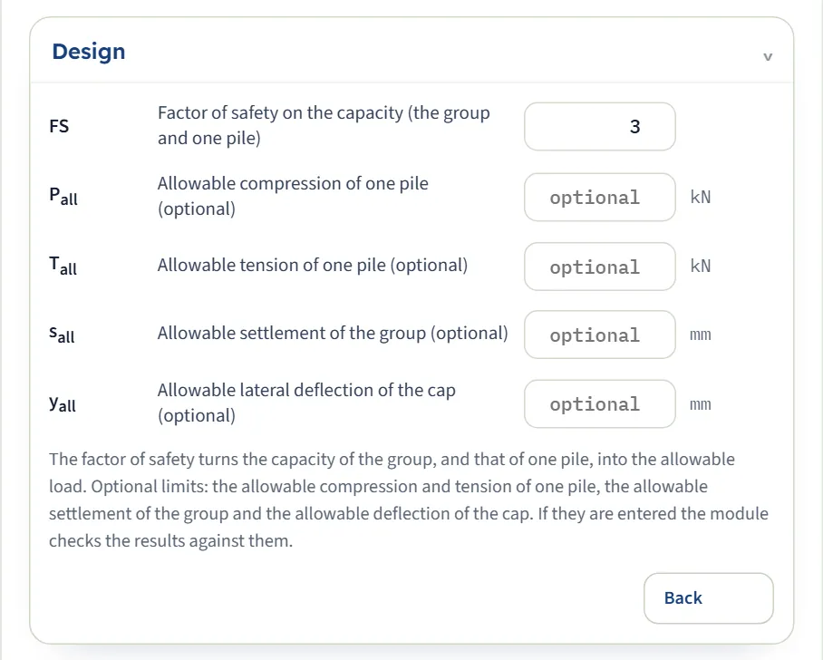
The factor of safety turns the capacity of the group, and that of one pile alone, into the allowable load. The four limits are optional: when entered, the module checks the results against them and says OK or NOT OK in words.
| Field | Symbol | Unit | Default | What to enter |
|---|---|---|---|---|
| Factor of safety on the capacity (the group and one pile) | FS | — | 3 | Factor of safety on the capacity of the group and on that of one pile. Accepted from 1 to 10. |
| Allowable compression of one pile (optional) | Pall | kN · tf · kip | empty | Allowable compression of one pile. If entered it is compared with the most loaded pile, and the lesser of this and Qu/FS governs. |
| Allowable tension of one pile (optional) | Tall | kN · tf · kip | empty | Allowable tension of one pile. Used when a pile is in tension; the lesser of this and Tu/FS governs. |
| Allowable settlement of the group (optional) | sall | mm · in | empty | Allowable settlement of the group. If entered, the settlement is given a verdict. Shown when settlement of the group is Calculated. |
| Allowable lateral deflection of the cap (optional) | yall | mm · in | empty | Allowable lateral deflection of the cap. If entered, the deflection is given a verdict. |
Choosing the methods and options
A handful of choices decide how the group is analysed. The tables below say what each one does, so that you can pick the one that fits your case and run another to compare.
Rectangular grid or triangular arrangement
| Rectangular grid | Triangular (equilateral) | |
|---|---|---|
| Inputs | nx, ny, sx, sy | nx, ny, one spacing s |
| Where the piles stand | Rows sx apart; piles of a row sy apart | Piles of a row s apart; rows s √3/2 apart; every second row shifted by s/2, so that every pile has its neighbours at s |
| Load on the piles | P = V/n + B x + C y | The same; the piles are not symmetric about the axes, so the two moments can be coupled through Σxy, and the Calculations tab shows the equation used |
| Efficiency in clay | Converse–Labarre with the spacing of each direction | The same equation written over the neighbouring pairs of piles, each pair at its own distance; it gives the rectangular form back for a grid |
| p-multipliers | From sx/D | From the spacing of the rows s √3/2 over D; the shift of the rows is not counted |
| Los Angeles and Seiler–Keeney equations | Printed beside Converse–Labarre for comparison | Not given |
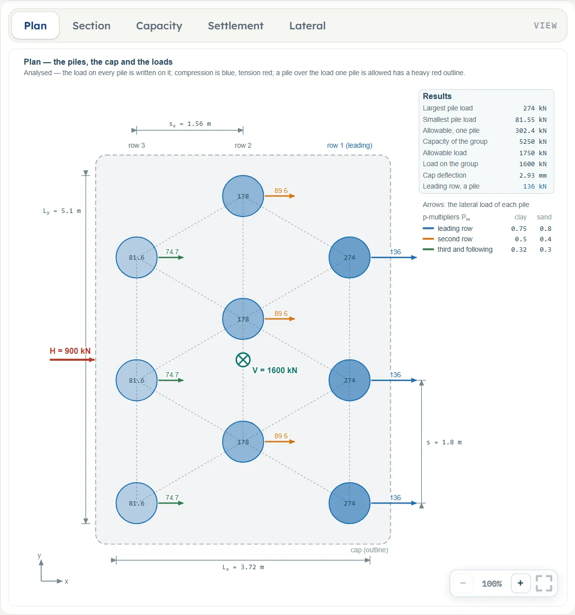
The Plan view of the triangular arrangement of the example, nine piles at s = 1.8 m: the rows are s √3/2 = 1.56 m apart and every second row is shifted by 0.9 m. Dashed lines join each pile to its neighbours. The rows are then closer than 3 pile widths, so the module cautions that the p-multipliers are beyond the range of the tests (see Messages).
Group efficiency: how much each pile loses
Piles close together share the soil between them and carry less than the sum of what each would carry alone. The module takes the efficiency layer by layer, by the kind of soil, and applies it to the shaft resistance of that layer; the base takes the efficiency of the layer it bears on:
| Layer | Efficiency used | Notes |
|---|---|---|
| Clay, any installation | Converse–Labarre: η = 1 − [(nx − 1) ny θx + (ny − 1) nx θy] / (90 nx ny), θ = tan⁻¹(D/s) | Estimated for friction piles in clay. The Los Angeles and Seiler–Keeney equations are printed for comparison and do not enter the capacity; the Seiler–Keeney equation, which takes the spacing in feet, is given from 2 ft. |
| Sand, driven or jacked | The chart of Kishida & Meyerhof at s/D | Never above 1. It is 1 up to φ′ = 40°, and between 40° and 45° it falls towards the curve of 45° of the chart. |
| Sand, bored | AASHTO LRFD: 0.65 at a spacing of 2.5 D, rising linearly to 1.0 at 4 D | The reduction for a shaft group in a cohesionless soil. |
The sand rules take one spacing, the least distance between two piles. The group then acts as Qind = n (Σ ηi Qs,i + ηb Qp), and the efficiency of the group on the Results tab is η = Qind / (n Qu).
Block failure
The piles and the soil between them may fail as one block of the plan size Lg × Bg and the depth of the piles. The block resists by the shear on its sides and by the bearing of its base:
- In a clay layer the shear is the undrained strength cu; in a sand layer it is the friction K0 σ′ tan φ′ on the vertical faces, with K0 = 1 − sin φ′.
- Where the base is in a clay, the bearing is cu N*c over the area of the block, with N*c read from the curves for L/Bg and Lg/Bg. Where the base is in a sand, it is the sum of the bases of the piles.
- The capacity of the group is the lesser of the piles as individuals and the block: Qg(u) = min(Qind, Qblock). The Capacity view shows both, and the Calculations tab says which one governs.
In the example the piles govern, 5,952 kN against 25,838 kN for the block. The block governs when the soil the group bears on is much weaker than the soil along its sides. As an illustration, take 12 × 12 piles at 2.5 D, 30 m long, in 4 m of sand (φ′ = 32°) over 26 m of stiff clay (cu = 150 kPa) over a soft clay (cu = 8 kPa), with the tips on the boundary of the two clays, V = 20,000 kN and no lateral load or moment. The piles with their efficiency give Qind = 322,484 kN, the block Qblock = 288,857 kN: the block governs, Qg(u) = 288,857 kN, and the Capacity view says “the block governs”.
One pile: the methods of each layer
The resistance of one pile alone is worked out in the Calculations tab, step 3, and none of it is typed. Every layer takes the method chosen for it, with its own numbers, and the base takes the method chosen in Point bearing for the soil the pile ends in. Each method is described in full in the manuals of Pile in sand, Pile in clay and Pile on layered soil; in short:
| Soil | Method | Unit skin friction f | Notes |
|---|---|---|---|
| Sand | K–δ method | f = K tan δ′ σ′, σ′ held constant below L′ = 15 D | K = K0 for a bored pile, 1.4 K0 for a driven or jacked one; δ′ = 0.75 φ′. |
| Sand | Coyle & Castello | f = K σ′ tan(0.8 φ′), on the mean σ′ of the layer | K from their chart at φ′ and L/D. Driven piles; refused for a bored pile, cautioned for a jacked one. |
| Clay | α method | f = α cu | Bored: the drilled-shaft α of O’Neill & Reese (0.55 up to cu/pa = 1.5, falling to 0.45 at 2.5), and no resistance over the top 1.5 m or the bottom 1 D. Driven or jacked: the driven-pile curve. |
| Clay | λ — extended | f = λ (σ′ + 2 cu) | λ read at the embedded length of the pile and applied layer by layer, an extension of the correlation. Driven piles; refused for a bored pile. |
| Clay | β method | f = (1 − sin φ′R) tan φ′R √OCR σ′ | Needs φ′R, the remoulded friction angle of your clay. |
| Method | Where | Unit resistance qp |
|---|---|---|
| Meyerhof | Sand | qp = σ′ N*q, limited to ql = 0.5 pa N*q tan φ′ |
| Meyerhof | Clay | qp = 9 cu |
| Vesic | Sand | qp = σ′o N*σ, σ′o = (1 + 2 K0) σ′ / 3; needs m = Es/pa |
| Vesic | Clay | qp = N*c cu, with N*c from the rigidity index Irr = 347 cu/pa − 33 (at most 300) |
| Coyle & Castello | Sand only | qp = σ′ N*q, N*q from their chart at L/D and φ′ |
| Reese & O’Neill | Bored pile, base in clay | qp = min[6 cub (1 + 0.2 L/D), 9 cub, 40 pa], cub the mean undrained strength over the 2 D below the base |
Settlement: calculated or left out
| Choice | What is worked out | What goes when it is left out |
|---|---|---|
| Calculated | Elastic: a pile at its working load V/n settles by the shortening of the pile, of its base and of its shaft (Vesic’s factors); the group settles Sg(e) = √(Bg/D) se. Needs Es. Consolidation: the load of the group spreads 2:1 from the depth 2L/3 and acts at the middle of every clay layer below it: Δσ′ = V / ((Bg + z) (Lg + z)), z the depth of the middle of the clay layer below 2L/3, ΔSc = Cc H / (1 + e0) log[(σ′o + Δσ′) / σ′o]; an over-consolidated clay settles less. | — |
| Not calculated | Nothing about the settlement. | The settlement step and its answers, the boxes e0, Cc, Cs, Es, νs, ξ and the allowable settlement, what the Settlement view draws and the drawing in the report. The loads, the capacity and the lateral response are unchanged. |
With Es left empty only the consolidation is calculated, and the card is labelled “(consolidation)”; with no clay layer below 2L/3 only the elastic part is.
The lateral group effect
A pile in a row behind another stands in the shadow of the pile in front, so its p–y curve is scaled by a p-multiplier that depends on the row. The module uses three: the leading row, the second row, and the third row and every row behind it, by the kind of soil in each layer:
- Sand layers: the multipliers of AASHTO LRFD, from the tests of Brown, Morrison & Reese and the centrifuge tests of McVay et al.: 0.8, 0.4 and 0.3 at a spacing of 3 D, 1.0, 0.85 and 0.7 at 5 D, interpolated between and rising to 1.0 at 8 D. Closer than 3 D the values of 3 D are used.
- Clay layers: Rollins et al. (2006), from full-scale tests in stiff clay: Pm = 0.26 ln(s/D) + 0.5 for the leading row, 0.52 ln(s/D) for the second and 0.60 ln(s/D) − 0.25 for the rest, none above 1.
- With one row in the direction of the load nothing shadows another pile, and every multiplier is 1.
| Spacing of the rows | Sand layers | Clay layers |
|---|---|---|
| 2 D | 0.80 / 0.40 / 0.30 | 0.68 / 0.36 / 0.17 |
| 3 D | 0.80 / 0.40 / 0.30 | 0.79 / 0.57 / 0.41 |
| 4 D | 0.90 / 0.63 / 0.50 | 0.86 / 0.72 / 0.58 |
| 6 D | 1.00 / 0.90 / 0.80 | 0.97 / 0.93 / 0.83 |
| Choice | Options | What it does |
|---|---|---|
| Pile heads | Held against rotation, Free to rotate (pinned) | A head held by the cap does not turn; a pinned head can. |
| Lateral loading | Static (sustained), Cyclic (repeated) | Static uses the p–y curves as they stand; cyclic uses the cyclic curves of API RP 2A. |
| Direction of the load | One direction (a leading row), Reversing (the mean of the rows) | One direction gives each kind of row its own multiplier; reversing gives every row the mean of the multipliers of the rows. |
Which should I pick?
- Set the installation first. It changes K, α, which methods are open and the efficiency of a sand layer.
- Start with the defaults for the methods: Meyerhof at the base, the K–δ method in sand and the α method in clay. Change one at a time and compare.
- Read the Capacity view. It shows whether the piles with their efficiency or the block govern, and how the efficiency changes with the spacing.
- Calculate the settlement when there is clay below the level 2L/3, including clay beside the lower shaft. The consolidation of the clays below the level 2L/3 is usually the larger part (the example: 76.66 mm of 84.60 mm).
- Leave the p-multipliers as they are unless you have test evidence for your soil and spacing; they are filled in from the spacing of the rows.
Analyze and read the results
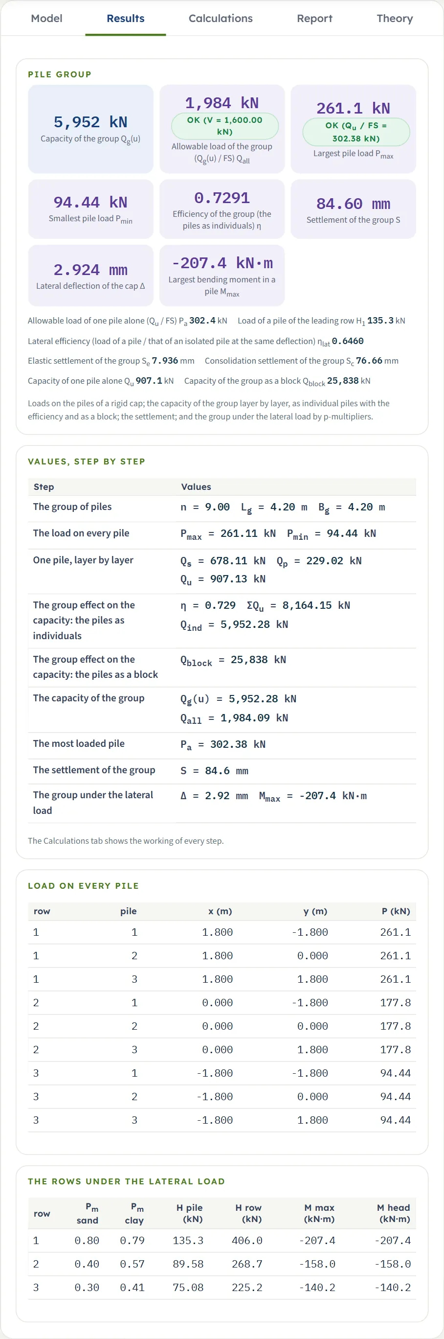
Press Analyze. The bar turns green, the inputs lock, and the Results tab shows its blocks, one below the other.
- Pile group. The cards with the main answers (the table below), and under them the lines of the secondary answers: the load one pile alone is allowed, the load of a pile of the leading row, the lateral efficiency, the elastic and the consolidation settlement, the capacity of one pile alone and that of the block.
- Values, step by step. One row for each step of the calculation, with its numbers.
- Load on every pile. A table of the row, the pile, its position x and y from the centroid of the group, and its load P. It is printed for a group of up to 40 piles.
- The rows under the lateral load. For each kind of row the p-multipliers of sand and clay, the lateral load of a pile and of the row, and the largest bending moment and the moment at the head of a pile.
The warnings and notes of the run, if there are any, are listed under the Warnings or Notes button on the green bar and printed in the report. The five views of the drawing now carry the numbers (see the screen).
The cards
| Card | What it is | Checked against |
|---|---|---|
| Capacity of the group Qg(u) | The lesser of the piles as individuals and the block | — |
| Allowable load of the group Qall | Qg(u) / FS | The vertical load V |
| Largest pile load Pmax | The load of the most loaded pile of the rigid cap | Qu/FS, the load one pile alone is allowed, or the allowable compression Pall if you entered it and it is smaller |
| Smallest pile load Pmin | The load of the least loaded pile. Negative: the pile is in tension, and the card is labelled “(tension)” | Only for a pile in tension: its tension capacity over FS, or Tall if smaller |
| Efficiency of the group η | Qind / (n Qu), for a group of more than one pile | — |
| Settlement of the group S | Elastic plus consolidation, or the one that is worked out | The allowable settlement sall, if entered |
| Lateral deflection of the cap Δ | Shown when the lateral load H is above zero | The allowable deflection yall, if entered |
| Largest bending moment in a pile Mmax | The largest moment found in a pile of any row, with its sign | — |
Compression and tension
Loads on the piles are positive in compression. A moment on the cap lifts the piles on its far side, and when the vertical load cannot balance it a pile goes into tension. In the Plan view such a pile is drawn in red, the card reads “Smallest pile load (tension)”, and the Notes list says which pile it is. The module then adds two checks, shown as two more lines under the cards:
- One pile in tension resists by its shaft alone: a clay layer by the same method as in compression, a sand layer at 0.75 of its resistance in compression. The most tension on a pile Tmax is checked against Tu/FS, or against Tall if you entered it and it is smaller.
- The piles in tension together are held by the lesser of their own shafts, each layer with the efficiency of its soil, and the block of soil that encloses them: the shear on its sides and its weight. Their sum ΣT is checked against Tg/FS.
The weight of the pile is not counted in tension. As an example, with My raised to 2700 kN·m the module gives Pmax = 427.8 kN and Pmin = -72.22 kN. The three piles of the back row are in tension (red); the three of the front row are over the load one pile alone is allowed (heavy outline), and the results box on the drawing adds the allowable tension.
The checks against allowable values
Where a limit applies, the card or the line carries a verdict in words, never by a colour alone, and the figure it was compared with in brackets:
| Verdict | Meaning |
|---|---|
| OK (V = 1,600.00 kN) | The value is within its limit. The example gives this on the allowable load of the group and, beside the largest pile load, “OK (Qu / FS = 302.38 kN)”. |
| OK, near the limit | The value is within the limit but above 90 % of it. |
| NOT OK | The value is over the limit. For the load on the group, the most loaded pile and the tension checks the module also raises a warning that says what to change; see Messages. |
Two checks are always made: the load on the group against its allowable load, and the most loaded pile against the load one pile alone is allowed. The tension checks are made when a pile is in tension. The settlement and the deflection of the cap are judged only when you enter sall and yall in the Design section; without them the numbers are given and not judged.
The Calculations tab, the report and the theory
The Calculations tab writes out the working in chapters: Given and what is sought, then one chapter per step, then Notes and assumptions. For this module the steps are:
- The group of piles — the plan size Lx, Ly of the group, Lg and Bg, and the spacing over the width.
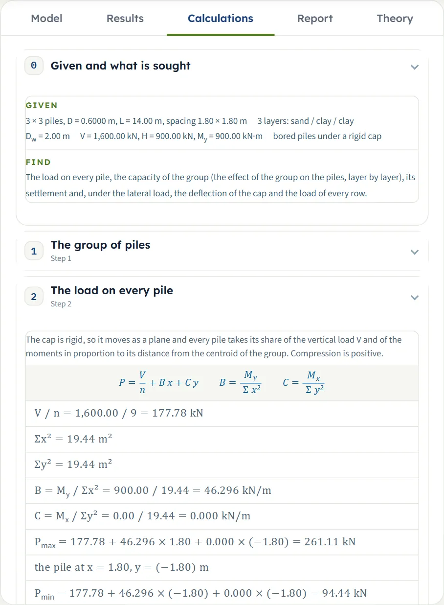
- The load on every pile — V/n, Σx², Σy², B and C, the largest and the smallest load, and the table of every pile.
- One pile, layer by layer — for each layer the method, its coefficients and f, Qs; the base with qp and Qp; and Qu.
- The group effect on the capacity: the piles as individuals — the efficiency of each layer, Qind and η.
- The group effect on the capacity: the piles as a block — the shear of each layer, the bearing of the base and Qblock.
- The capacity of the group — Qg(u), which one governs, Qall and the share of it that V takes.
- The most loaded pile — Pmax against Qu/FS (for a group of more than one pile).
- The settlement of the group — the elastic settlement of a pile and of the group, the consolidation of each clay layer, and the total.
- The group under the lateral load — the p-multipliers, the deflection of the cap, the load of each row and the moments.
A chapter appears only when it applies: the settlement chapter when the settlement is calculated, the lateral chapter when H is above zero, and The piles in tension, with its own checks, after step 7 when a pile is in tension; it then becomes step 8, the settlement step 9 and the lateral load step 10. Notes and assumptions lists what the run took for granted, such as the drilled-shaft rule for a bored pile or the rigid cap. Every number on the Results tab can be traced to a step here.
The report
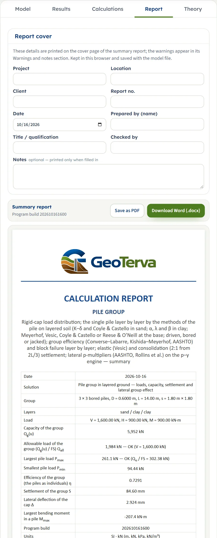
The Report tab turns the same working into a summary report. Fill in the cover (project, location, client, report number, date, prepared by, title, checked by, notes) and press Save as PDF or Download Word (.docx). The report has seven parts: 1 Introduction and scope, 2 Input data, 3 Calculation (one part for each step, 3.1 to 3.9, and 3.10 when a pile is in tension), 4 Results, 5 Assumptions and notes, 6 Summary and 7 References. It carries the drawings of the views that were worked out, and the units line states the conversion constants.
The theory
The Theory tab explains the method in fifteen chapters: 1 A group of piles; 2 The load on every pile; 3 The single pile; 4 The efficiency of the group; 5 Piles in sand; 6 Layer by layer; 7 Block failure; 8 Elastic settlement; 9 Consolidation settlement; 10 Lateral load: the p-multipliers; 11 Solving the group; 12 Reading the results; 13 A worked example, whose numbers are computed by the module’s own code; 14 What the module assumes; 15 References.
Worked example: the module’s own example
The module opens on this example. Reset to defaults brings it back at any time, so you can follow the numbers on your own screen.
| Section | Input | Value |
|---|---|---|
| Group | Arrangement, rows, piles in a row, spacings | Rectangular grid, nx = 3 rows of ny = 3 piles, sx = sy = 1.8 m (3 D) |
| Pile | Section, installation | Circular, solid; bored |
| Pile | Size, stiffness, length, cap | D = 0.6 m, Ep = 30 000 MPa, fEI = 1, L = 14 m; base of the cap at the ground (zc = e = 0) |
| Soil layers | Layer-1 | Sand, H = 4 m, γ = 18 and γsat = 19 kN/m³, φ′ = 32° |
| Soil layers | Layer-2 | Clay, H = 6 m, γ = 18 and γsat = 19 kN/m³, cu = 50 kPa, e0 = 0.9, Cc = 0.28, OCR = 1 |
| Soil layers | Layer-3 | Clay, H = 8 m, γ = 18 and γsat = 19 kN/m³, cu = 90 kPa, e0 = 0.7, Cc = 0.2, OCR = 1 |
| Groundwater | Water table | Present, Dw = 2 m |
| Loading | Loads at the base of the cap | V = 1600 kN, H = 900 kN, My = 900 kN·m, Mx = 0 |
| Point bearing | Method | Meyerhof |
| Skin friction | Methods, coefficients | Layer-1 K–δ, K = 0.47 and δ′ = 24° (filled in); Layer-2 and Layer-3 α method, α = 0.55 (filled in) |
| Settlement | Choice, soil below the base | Calculated; Es = 30 MPa, νs = 0.3, ξ = 0.6 |
| Lateral group effect | Heads, loading, direction | Held against rotation; static; one direction. The multipliers are filled in from sx/D = 3 |
| Design | Factor of safety; limits | FS = 3; no limits |
Step 1: the load on every pile
V/n = 1600/9 = 177.78 kN. The piles stand at x = +1.8, 0 and −1.8 m from the centroid, so Σx² = 3 × (1.8² + 0 + 1.8²) = 19.44 m² and B = My/Σx² = 900/19.44 = 46.296 kN/m. The front row takes 177.78 + 46.296 × 1.8 = 261.11 kN a pile, the middle row 177.8 kN and the back row 177.78 − 46.296 × 1.8 = 94.44 kN. The three rows add to 3 × (261.11 + 177.78 + 94.44) = 1600 kN: the moment only moves load from the back to the front.
Step 2: one pile, layer by layer
The perimeter is π × 0.6 m and the area of the base 0.2827 m². The pile is bored, so K stays at K0 and the clay layers take the drilled-shaft α.
- Layer-1, sand 0–4 m, K–δ. K = 1 − sin 32° = 0.470, δ′ = 0.75 × 32° = 24°. The critical depth L′ = 15 D = 9 m is not reached in the layer, so the mean effective stress of the layer, 31.60 kPa (the water table is at 2 m), is used: f = 0.470 × tan 24° × 31.60 = 6.61 kPa, which over the shaft of the layer gives Qs = 49.85 kN.
- Layer-2, clay 4–10 m, α. α = 0.55: f = 0.55 × 50 = 27.50 kPa and Qs = 27.50 × π × 0.6 × 6 = 311.02 kN.
- Layer-3, clay 10–14 m, α. f = 0.55 × 90 = 49.50 kPa, but the drilled-shaft rule leaves out the bottom 1 D = 0.6 m of the shaft, so the friction acts over 3.40 m of the 4.00 m: the mean is 49.50 × 3.40/4.00 = 42.08 kPa and Qs = 317.24 kN.
- Base, in Layer-3, Meyerhof. qp = 9 cu = 9 × 90 = 810 kPa and Qp = 810 × 0.2827 = 229.02 kN.
Qu = 49.85 + 311.02 + 317.24 + 229.02 = 907.13 kN. The load one pile alone is allowed is Qu/FS = 907.13/3 = 302.38 kN; the most loaded pile takes 261.11 kN, 86 % of it.
Step 3: the efficiency and the block
- Clay layers. θ = tan⁻¹(0.6/1.8) = 18.43° in both directions, so η = 1 − [2 × 3 × 18.43 + 2 × 3 × 18.43] / (90 × 3 × 3) = 0.727.
- Sand layer, bored. At s/D = 3 the AASHTO rule gives 0.65 + 0.35 × (3 − 2.5)/(4 − 2.5) = 0.767.
- As individuals. Qind = 9 × (0.767 × 49.85 + 0.727 × (311.02 + 317.24 + 229.02)) = 5,952.28 kN, so the group acts as 5,952.28/8,164.15 = 0.729 of the sum of its piles.
- As a block. Lg = Bg = (3 − 1) × 1.8 + 0.6 = 4.20 m, perimeter 16.80 m. The sides give 623.66 + 5,040.00 + 6,048.00 = 11,711.7 kN (τ = K0 σ′ tan φ′ = 9.28 kPa in the sand, cu in the clays); the base gives 4.20 × 4.20 × 90 × N*c, with N*c read from the curves as 8.90 (to two decimals), 14,126.5 kN; Qblock = 25,838 kN.
Step 4: the capacity of the group
Qg(u) = min(5,952.28, 25,838.1) = 5,952.28 kN: the piles with their efficiency govern, and the block is far from it. Qall = 5,952.28/3 = 1,984.09 kN, against the V = 1,600 kN the group carries: 81 % of it, OK.
Step 5: the settlement
- Elastic. A pile at its working load V/n = 177.78 kN, 75 % of it on the shaft, settles se = 0.2057 + 2.456 + 0.3383 = 3.000 mm (shortening of the pile, base, shaft). The group, wider, settles √(Bg/D) = √(4.20/0.60) times as much: Sg(e) = 7.936 mm.
- Consolidation. The load spreads 2:1 from 2L/3 = 9.33 m. Layer-2 has 0.6667 m below that level; its middle is 0.333 m below it, where Δσ′ = 1600/((4.20 + 0.333) × (4.20 + 0.333)) = 77.85 kPa on σ′o = 106.46 kPa, which settles it 23.4 mm. Layer-3, 8 m thick, has its middle 4.67 m below the level, where Δσ′ = 20.35 kPa on σ′o = 146.28 kPa: 53.2 mm. Sc = 76.66 mm.
- Total. S = 7.936 + 76.66 = 84.60 mm.
Step 6: the lateral load
The rows are 1.8 m = 3 D apart, so the multipliers are, for the leading, second and third row: sand 0.80, 0.40 and 0.30; clay 0.79, 0.57 and 0.41. The cap deflects Δ = 2.92 mm, at which a pile of the three rows carries 135.3, 89.58 and 75.08 kN, so the rows carry 406.0 + 268.7 + 225.2 = 900 kN = H. An isolated pile under H/n = 100 kN would deflect 1.85 mm; the group deflects 1.58 times as much, and a pile of it takes 65 % of what an isolated pile takes at the same deflection (ηlat = 0.646). The largest moment, −207.4 kN·m, is at the head of a pile of the leading row.
How each input changes the answer
Each row below changes one thing in the example and runs the module again. The numbers are the results the module gives, in kN and mm, so you can reproduce any row; a dash means the module gives no such result in that run. The last column says what changes, and where a check fails or comes within 10 % of its limit (the allowable load of the group against V, Pmax against Qu/FS).
| Change | Qu (kN) | η | Qg(u) (kN) | Pmax (kN) | S (mm) | Δ (mm) | What happens |
|---|---|---|---|---|---|---|---|
| The default example | 907.1 | 0.7291 | 5,952 | 261.1 | 84.60 | 2.924 | The reference |
| Spacing 2.4 m (4 D) | 907.1 | 0.8035 | 6,560 | 240.3 | 66.96 | 2.379 | η rises; the longer lever arm lowers Pmax; the multipliers rise |
| Spacing 3.6 m (6 D) | 907.1 | 0.8675 | 7,083 | 219.4 | 47.35 | 1.981 | η 0.87; the multipliers are 1.0 to 0.8 in sand and 0.97 to 0.83 in clay |
| Spacing 1.2 m (2 D) | 907.1 | 0.6088 | 4,971 | 302.8 | 113.0 | 2.955 | Under 2.5 D: η falls, the lever arm shortens, Pmax is over its limit and Qall is within 10 % of V |
| 4 rows of 3 piles | 907.1 | 0.7129 | 7,761 | 183.3 | 68.65 | 2.305 | Twelve piles: V/n and Pmax fall, η falls a little |
| 2 rows of 3 piles | 907.1 | 0.7613 | 4,144 | 433.3 | 108.7 | 4.003 | Six piles: Pmax is over its limit and Qall is below V |
| Triangular arrangement, s = 1.8 m | 907.1 | 0.6430 | 5,250 | 274.0 | 80.92 | 2.934 | Rows 1.56 m apart, so the lever arm is shorter and Pmax is within 10 % of its limit; the neighbouring pairs lower η |
| V = 1200 kN | 907.1 | 0.7291 | 5,952 | 216.7 | 65.18 | 2.923 | Pmin falls to 50.00 kN; the settlement falls with the load |
| V = 2400 kN | 907.1 | 0.7291 | 5,952 | 350.0 | 121.0 | 2.925 | Pmax is over its limit and Qall is below V |
| My = 0 | 907.1 | 0.7291 | 5,952 | 177.8 | 84.60 | 2.924 | Every pile takes V/n; the capacity and the lateral result do not change |
| My = 2700 kN·m | 907.1 | 0.7291 | 5,952 | 427.8 | 84.60 | 2.924 | A pile goes into tension, Pmin negative; Pmax is over its limit |
| H = 450 kN | 907.1 | 0.7291 | 5,952 | 261.1 | 84.60 | 1.416 | Half the load, 0.48 of the deflection |
| H = 1350 kN | 907.1 | 0.7291 | 5,952 | 261.1 | 84.60 | 4.577 | 1.5 times the load, 1.57 times the deflection |
| Settlement not calculated | 907.1 | 0.7291 | 5,952 | 261.1 | — | 2.924 | Nothing else changes |
| Driven piles | 1,030 | 0.7455 | 6,908 | 261.1 | 83.85 | 2.924 | K = 1.4 K0 and the driven-pile α; the sand has η = 1 below φ′ = 40°. A jacked pile gives the same figures |
| No water table | 914.1 | 0.7294 | 6,000 | 261.1 | 55.41 | 2.917 | The sand and the clays carry more effective stress; the consolidation falls |
| L = 10 m | 558.8 | 0.7304 | 3,673 | 261.1 | 129.8 | 2.924 | Base on the boundary of Layer-2 and Layer-3; Qall is below V and Pmax is over its limit; the spread starts higher and the settlement rises |
| L = 16 m | 1,094 | 0.7287 | 7,173 | 261.1 | 66.68 | 2.924 | More shaft in Layer-3; less settlement |
| D = 0.8 m | 1,286 | 0.6453 | 7,471 | 261.1 | 79.34 | 1.836 | Spacing now 2.25 D, under 2.5 D; stiffer piles deflect less |
| Base by Vesic | 968.6 | 0.7289 | 6,354 | 261.1 | 85.78 | 2.924 | Only Qp changes; Reese & O’Neill gives the figures of the default, held at 9 cub |
| FS = 2.5 | 907.1 | 0.7291 | 5,952 | 261.1 | 84.60 | 2.924 | Only Qall and the limit on Pmax move |
| Pile heads free to rotate | 907.1 | 0.7291 | 5,952 | 261.1 | 84.60 | 8.494 | The head can turn: the cap deflects 2.9 times as much |
| Cyclic lateral loading | 907.1 | 0.7291 | 5,952 | 261.1 | 84.60 | 3.045 | The API cyclic curves are used; the cap deflects a little more |
| Reversing lateral load | 907.1 | 0.7291 | 5,952 | 261.1 | 84.60 | 2.859 | Every row takes the mean multiplier; the cap deflects a little less |
| Clay layers over-consolidated, OCR = 3 | 907.1 | 0.7291 | 5,952 | 261.1 | 23.27 | 2.924 | The consolidation falls from 76.66 to 15.33 mm |
| Layer-3 softer, cu = 60 kPa | 725.0 | 0.7296 | 4,761 | 261.1 | 83.56 | 2.924 | Qu falls; Qall is below V and Pmax is over its limit |
| Driven, clay layers by the λ method | 1,214 | 0.7426 | 8,116 | 261.1 | 83.01 | 2.924 | λ is read at the length of the pile |
| Driven, clay layers by the β method | 845.0 | 0.7495 | 5,700 | 261.1 | 85.06 | 2.924 | φ′R = 30°, the box’s default; Pmax is within 10 % of its limit |
Read across the table for what each input does. The resistance of one pile (Qu) depends on the length, the diameter, the installation, the methods and the soil, and not on the group. The efficiency follows the spacing, the arrangement and the installation. The load on the piles follows the number of piles, the lever arm of the moment and the loads. The settlement follows the load, the water table, the length and the clay parameters. The lateral result follows the lateral load, the spacing of the rows, the heads, the loading and the stiffness of the piles.
Messages: stops, warnings and notes
The module tells you in plain words when something prevents the calculation, when a result needs care, and what it assumed. There are three kinds, and each message names the fields it concerns and says what to do.
- A stop is a window titled “Cannot analyse” (the bar turns brown). Nothing is calculated until you change the inputs marked in red.
- A warning is a caution raised by a run: the results are there, and they need care or fail a check. The Warnings button on the green bar lists them.
- A note states what the run took for granted. The button on the green bar reads Notes when there are no warnings, and the window is titled “Notes and assumptions”.
| Kind | When | Message and what to do |
|---|---|---|
| Stop | The layers do not reach the pile tips | “The layers must reach the pile tip. They reach 18.00 m, the pile tip is at 20.00 m.” Add a layer, or thicken the last one. |
| Stop | One row of piles, or one pile in a row, with the moment across it | “The piles stand in a line and cannot take a moment across it.” Add a row or a pile on the other side, or remove that moment. |
| Stop | The λ method in a bored pile | “Change the skin-friction method of Layer-2. The λ method was read from piles driven in clay; a bored pile is outside it.” Use the α or β method in a clay. |
| Stop | Coyle & Castello in a bored pile | “Change the skin-friction method of Layer-1. Coyle & Castello is calibrated on piles driven in sand; a bored pile is outside it.” Use the K–δ method in a sand. |
| Stop | Vesic at the base in a weak clay | “Change the point-bearing method. Vesic’s rigidity index Irr = 347 (cu/pa) − 33 has no value at cu = 5.0 kPa in Layer-3; the correlation starts at about 9.8 kPa.” Use Meyerhof for the base (qp = 9 cu). |
| Stop | The base of the cap given both below and above the ground | “The base of the cap is either below the ground or above it.” Enter zc or e, not both. |
| Stop (input error) | A value outside what the field accepts, for example 101 rows or φ′ = 19° | “Rows in the direction of the lateral load (nx) must be at most 100.” and “Friction angle (20–45°) (φ′1) must be at least 20°.” Correct the field marked in red. |
| Stop | A lateral load more than the group can resist (H = 20,000 kN on the example) | “The lateral load is more than the group can resist: no equilibrium.” The window adds that the rows together carry about 16,092 kN at most, at a deflection of the cap of 2,940 mm (4.9 pile widths). Lower the load, or lengthen or stiffen the piles, or widen the spacing. |
| Warning | A spacing under 2.5 pile widths | “The spacing of the piles is 2.00 pile widths, less than the 2.5 the source gives as the least.” Widen the spacing. |
| Warning | Rows closer than 3 pile widths, which includes a triangular group at s = 3 D, whose rows are 2.6 D apart | “The rows are closer than 3 pile widths: the p-multipliers are beyond the range of the tests.” Widen the spacing of the rows, or judge the result accordingly. |
| Warning | The load on the group over its allowable load | “The load on the group, 6,500.00 kN, exceeds its allowable load 1,984.09 kN.” Lengthen or widen the piles, add piles or widen the spacing. |
| Warning | The most loaded pile over what one pile alone is allowed | “The most loaded pile takes 427.78 kN, more than the 302.38 kN one pile alone is allowed.” Lengthen or widen the piles, add piles, or place them further from the centre of the group in the direction of the moment. |
| Warning | A pile in tension over its allowable tension (here Tall = 50 kN) | “The most tension on a pile, 72.22 kN, is more than the 50.00 kN one pile is allowed in tension.” Lengthen the piles, add piles, widen the group in the direction of the moment, or increase the vertical load that holds them down. |
| Warning | Coyle & Castello in a jacked pile | “Coyle & Castello is for driven piles; this one is jacked.” Read the result as an estimate, or use the K–δ method. |
| Warning | The λ method in a driven or jacked pile | “The λ method is applied layer by layer here, which is an extension of it.” Read the λ layers as an estimate, or use α or β for a layered profile. A jacked pile raises a second warning, “The λ method is for driven piles; this one is jacked.” |
| Warning | K too high for a bored pile | “K = 1.20 in Layer-1 is too high for a bored pile.” Use K ≈ K0, or say why this shaft carries more. |
| Warning | A cap deflection over a fifth of the pile width (H = 9000 kN on the example) | “The cap deflects 329 mm, more than a fifth of the pile width.” The p–y curves are carried beyond the deflections they were derived for, and the result is an estimate. Lower the lateral load, or lengthen or stiffen the piles, or widen the spacing. |
| Note | A pile in tension | “The pile at x = -1.80 m is in tension, 72.22 kN.” Its shaft resistance in tension, and the piles in tension together against their block, are checked. |
| Note | A cap deflection over a tenth of the pile width | “The deflection of the cap is more than a tenth of the pile width.” The p–y curves were derived for deflections up to a few per cent of the width; compare the deflection with what the structure can bear. |
| Note | The base exactly on a layer boundary | “Computed with the base bearing on Layer-3, the layer below the level the base sits on.” The point resistance is worked from the soil beneath the base; the layer above it gives shaft friction only. |
| Note | The profile ends within 2 D of the tips | “Computed with the deepest layer taken to continue below 18.00 m.” The last layer is taken to continue with the same properties. |
| Note | A bored pile | “Computed with the drilled-shaft α of O’Neill & Reese in Layer-2, Layer-3.” and “Computed with the base taken as clean and the clay of Layer-3 beneath it undisturbed.” No reduction is applied for the bored construction. |
| Note | Every run | “The cap is taken as rigid.” and “The group effect is worked out layer by layer, by the kind of soil in each layer.” A cap below the ground adds “The soil above the base of the cap acts in the stresses of the axial analysis.”; cyclic loading adds “Cyclic loading: the API cyclic curves are used.” |
The warnings and notes of the run are printed in the report, in its part 5, Assumptions and notes, so the reader of the report sees the same assumptions you saw.
Good practice and common mistakes
- Enter V as the net load with the weight of the cap, and the loads at the base of the cap. A lateral load at a height h above the base of the cap is H and the moment My = H h. Mind the sign: a positive My puts more compression on the side the lateral load pushes towards.
- Keep the spacing at 3 pile widths or more where you can. The module flags a spacing under 2.5 D for the capacity, and a spacing of the rows under 3 D for the lateral part, where the multipliers are outside the range of the tests. The what-if table shows what the spacing does to η, Pmax and Δ.
- Look at the most loaded pile, not only at the group. The group can be within its capacity while the pile on the side of the moment is over what one pile alone is allowed. The card Pmax and its verdict are there for this.
- Describe the ground below the tips. The layers must reach the tips, and the base resistance comes from the soil at and just below them. Take the profile to at least 2 D below the tips, or accept the module’s note that the last layer continues.
- Match the installation to the pile. It decides K, α, which methods are open and the efficiency of a sand layer. A driven pile modelled as bored under-predicts the shaft; a bored pile modelled as driven over-predicts it.
- Read the Capacity view. It shows whether the piles with their efficiency or the block govern, and where your spacing stands on the efficiency curves.
- Take the settlement from clay parameters you trust. The consolidation of the clays below the level 2L/3 is usually the larger part of the settlement. OCR = 1 is the safe side; an over-consolidated clay settles much less (the what-if table: 23.3 mm with OCR = 3 against 84.6 mm).
- Treat a large cap deflection with care. The p–y curves were derived for deflections of a few per cent of the width. The module notes a deflection above a tenth of the pile width and cautions above a fifth.
- Do not edit the p-multipliers without evidence. They follow the spacing of the rows; type over them only for a soil and a spacing you have test results for.
- Compare variants. Keep each run with Quick Save…: two lengths, two spacings, bored and driven. Load brings any of them back.
- Check the units after you switch the system: type values in the units shown beside the boxes.
- Read the notes. They list what the module assumed and are printed in the report.
Frequently asked questions
How do I calculate the load on each pile of a pile group under a moment?
For a rigid cap each pile takes its share of the vertical load plus a part of the moment in proportion to its distance from the centroid of the group: P = V/n + My x / Σx² + Mx y / Σy² for a symmetric grid, compression positive. In GeoTerva’s Pile group module you enter V, H, My and Mx at the base of the cap and the module lists the load on every pile, with the largest and the smallest. In the module’s example, 1600 kN and 900 kN·m on 3 × 3 piles at 1.8 m give 261.1, 177.8 and 94.44 kN on the three rows.
What is the group efficiency of a pile group and how does the module estimate it?
The efficiency η is the capacity of the piles acting in the group divided by the sum of what each would carry alone. The module takes it layer by layer, by the kind of soil: Converse–Labarre for a clay layer, the chart of Kishida & Meyerhof (never above 1) for a driven or jacked pile in sand, and the AASHTO LRFD reduction (0.65 at 2.5 diameters rising to 1.0 at 4) for a bored pile in sand. In the example, at a spacing of 3 diameters, the group acts as 0.729 of the sum of its piles.
When does block failure govern the capacity of a pile group?
The module works out the group also as one block of soil and piles, of the plan size of the group and the depth of the piles, resisting by the shear on its sides and the bearing of its base, and takes the lesser of the block and the piles as individuals with their efficiency. The block governs when the soil the group bears on is much weaker than the soil along its sides: 12 × 12 piles at 2.5 diameters, 30 m long, in 4 m of sand over 26 m of stiff clay (cu = 150 kPa) over a soft clay (cu = 8 kPa), with the tips on the boundary of the two clays, a vertical load of 20,000 kN and no lateral load or moment, give 322,484 kN as individuals and 288,857 kN as a block, so the block governs. In the module’s default example the piles govern, 5,952 kN against 25,838 kN for the block. The Capacity view draws both and says which governs.
What spacing should I use between the piles of a group?
The module flags a centre-to-centre spacing under 2.5 pile widths, where the methods are outside their experience, and a spacing of the rows under 3 widths for the lateral part, where the p-multipliers are beyond the range of the tests. Wider spacing raises the efficiency, lengthens the lever arm of the moment and raises the p-multipliers. On the module’s example, 1.2 m (2 D) gives η = 0.6088 and 3.6 m (6 D) gives 0.8675.
How does the module check a pile in tension?
When the moment lifts the piles on the far side of the cap, the smallest load is negative and the card reads “Smallest pile load (tension)”. A pile in tension resists by its shaft alone: a clay layer as in compression, a sand layer at 0.75 of its resistance in compression, with the weight of the pile left out. The most tension on a pile is checked against its tension capacity over the factor of safety, and the piles in tension together against the lesser of their shafts and the block of soil around them.
How is the settlement of a pile group calculated?
In two parts. The elastic settlement of a pile at its working load, by Vesic’s method, is multiplied by the square root of the width of the group over the pile diameter. The consolidation settlement spreads the load of the group 2 vertical to 1 horizontal from a level 2L/3 below the top of the piles and settles every clay layer below it under the stress at its middle, from e0, Cc and OCR. In the example they are 7.936 mm and 76.66 mm, 84.60 mm in all.
Can I leave the settlement out?
Yes. Choose Not calculated in the Settlement section. The settlement step, the clay parameters e0, Cc and Cs, Es, νs, ξ, the allowable settlement and the Settlement view are left out; the loads, the capacity and the lateral response are worked out as before. The Settlement view button stays and says that the settlement of the group is not calculated. Leaving Es empty leaves out only the elastic part. With H = 0 the Lateral view says that no lateral load is given.
How does the module handle a lateral load on a pile group?
The cap is rigid, so every pile head has the same deflection. The p–y curve of every layer of a pile is scaled by the p-multiplier of its row (AASHTO LRFD for a sand layer, Rollins et al. 2006 for a clay layer), so the leading row, which the load pushes towards, takes more than the rows in its shadow. The module finds the deflection of the cap at which the rows carry the load together and gives the load and the moment of every row. In the example 900 kN deflects the cap 2.92 mm, and the leading row takes 135.3 kN a pile against 75.08 kN for the third row.
What do the p-multipliers mean and can I change them?
A p-multiplier is the factor by which the soil reaction of a pile in a group is reduced because it stands behind another pile. The module uses one for the leading row, one for the second row and one for the third row and those behind it, separately for sand and for clay layers, filled in from the spacing of the rows. You can type over any of them; emptying the box returns the module’s value.
Can I use a triangular arrangement of piles?
Yes. Choose Triangular (equilateral) in the Group section and enter one spacing: the piles of a row are that far apart, the rows are 0.866 of it apart (√3/2) and every second row is shifted by half of it. The efficiency of a clay layer is written over the neighbouring pairs of piles, the p-multipliers follow the spacing of the rows, and the block is the rectangle that encloses the piles.
What changes between driven, bored and jacked piles in a group?
Installation decides which methods are open (Coyle & Castello and the λ method are refused for a bored pile), what the boxes are filled in with (K about K0 for a bored pile and 1.4 K0 for a driven or jacked one; α from the drilled-shaft rule for a bored pile) and the efficiency of a sand layer. On the module’s example, driven piles give a single-pile capacity of 1,030 kN against 907.1 kN for bored piles, and a jacked pile gives the same figures as a driven one.
Do I have to enter the capacity of a single pile?
No. The module works the resistance of one pile out from the ground, layer by layer, by the methods of the pile on layered soil, and none of it is typed. Each layer takes the method you choose for it, and the base takes the method you choose in the Point bearing section.
What do OK, NOT OK and OK, near the limit mean on the results?
They are the verdicts of the checks against allowable values, written in words with the figure compared in brackets. OK means the value is within its limit, OK, near the limit means it is within the limit but above 90 % of it, and NOT OK means it is over. The module checks the load on the group against its allowable load, the most loaded pile against the load one pile alone is allowed, a pile in tension against its tension capacity, and, when you enter the limits, the settlement and the deflection of the cap.