

What the module calculates
Seismic bearing capacity gives the ultimate and the allowable bearing pressure of a strip (continuous) footing on a c–φ soil while an earthquake acts on it, by the theory of Richards, Elms and Budhu (1993). The failure mechanism is two Coulomb wedges: an active wedge under the footing and a passive wedge beside it, with the wall friction δ = φ/2 on the vertical face between them. The earthquake enters as a pseudo-static body force, the horizontal seismic coefficient kh (and, if you wish, the vertical one kv), which tilts the resultant of weight and inertia by the angle θ and makes the wedges shallower.
The factors come in closed form, once for the static case and once for the earthquake. The ultimate bearing capacity is the same sum of three terms in both:
with the surcharge q = γ Df of the soil above the base, and θ = tan⁻¹[kh / (1 − kv)]. The allowable pressures and the check of your applied pressure are built on the seismic capacity quE; the static value qu of the same wedges is reported beside it, so you see what the earthquake takes away.
What you can describe
- A strip footing of width B founded at the depth Df, on one soil below the footing described by c, φ and γ.
- The earthquake by kh (0 to 0.8) and kv (0 to 0.5).
- A factor of safety FS for the allowable pressures, and an optional applied vertical gross pressure qapplied that the module checks (PASS or FAIL).
The module draws the two wedges to scale under the footing, shows the capacity as bars, plots the three factors against φ, writes out every step, and prepares a PDF or Word report.
What belongs to other modules
- Static design of footings. Terzaghi for general and local shear, with a water table; Meyerhof for strip, square, rectangular and circular footings with shape, depth and inclination factors; Hansen and Vesic for sloping ground, a tilted base and an inclined load. The static value this module prints is the capacity of its own two-wedge mechanism, not the classical Prandtl-type value those four give.
- Undrained clay with φ = 0. The wedges need a friction angle; the module stops for φ = 0 and points to Terzaghi or Meyerhof.
- An independent horizontal force, a moment or an eccentricity of the footing. The inertia of the soil is already carried by kh, so no separate horizontal load is entered here; for those effects use a method with inclination factors (Meyerhof, Hansen, Vesic).
- The earth pressure on a wall in an earthquake: Mononobe–Okabe.
Before you start: what you need
Have these ready from your design:
| What | Notes |
|---|---|
| The footing width B and the founding depth Df | Your design. A continuous footing: B is its width. Df is the depth of the base below the ground surface, zero or more. |
| The cohesion c, friction angle φ and unit weight γ | Tests or correlations. The soil below the base. φ must be above zero for the analysis to run, and the module accepts up to 50°. |
| The seismic coefficients kh and kv | Your seismic design. The module takes the values you enter. kh is the horizontal coefficient, kv the vertical one; with kv = 0 only the horizontal inertia acts. |
| A factor of safety FS | Your design. At least 1. The allowable pressures are the capacity divided by it. |
| The applied pressure qapplied (optional) | Your structural analysis. The vertical gross pressure at the base, V/A: the column load together with the weight of the footing and of the soil above it, divided by the base area, from service loads. |
Quick start in eight steps
- Open the module and choose the units
Open Seismic bearing capacity from the Bearing Capacity family. Pick SI · kN, SI · tf or US in the header; you can change it at any time, even after Analyze.
- Describe the footing
In Footing enter the width B and the founding depth Df. The shape is fixed to Strip (continuous).
- Describe the soil
In Soil enter c, φ and γ of the soil below the footing.
- Enter the applied pressure (optional)
In Loads enter qapplied to have the footing checked; leave it blank to get the capacity only.
- Set the factor of safety
In Analysis Settings enter FS.
- Enter the earthquake
In Earthquake enter the horizontal seismic coefficient kh and the vertical one kv.
- Press Analyze
Press Analyze at the foot of the Model tab. The bar reads Analysed, the inputs lock, and a window lists the warnings, if any. The module stays on the Model tab; the result is on the Results tab.
- Read the answer, the working and the report
The Results tab gives quE (gross and net), the allowable pressures, the static capacity and the design check; the Section, Capacity and Factors buttons change the drawing. Calculations shows every step, Report saves a PDF or Word file, Theory derives the method.
The screen: section, capacity and factors
The layout is the one every GeoTerva module shares, described in the workspace guide. The drawing on the left has three views, chosen with the buttons above it, and the five tabs Model, Results, Calculations, Report and Theory are on the right.
Section: the footing and the two wedges
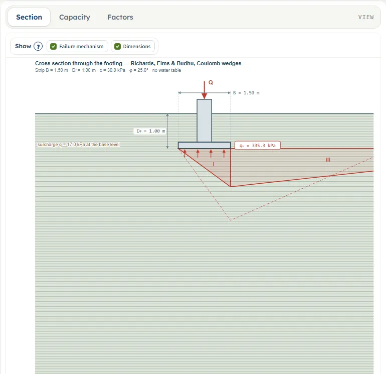
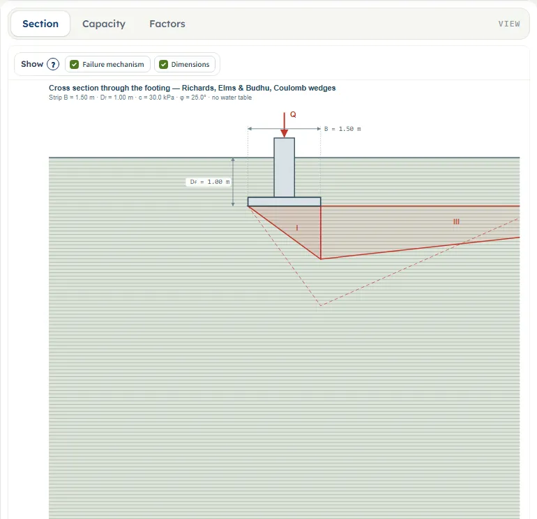
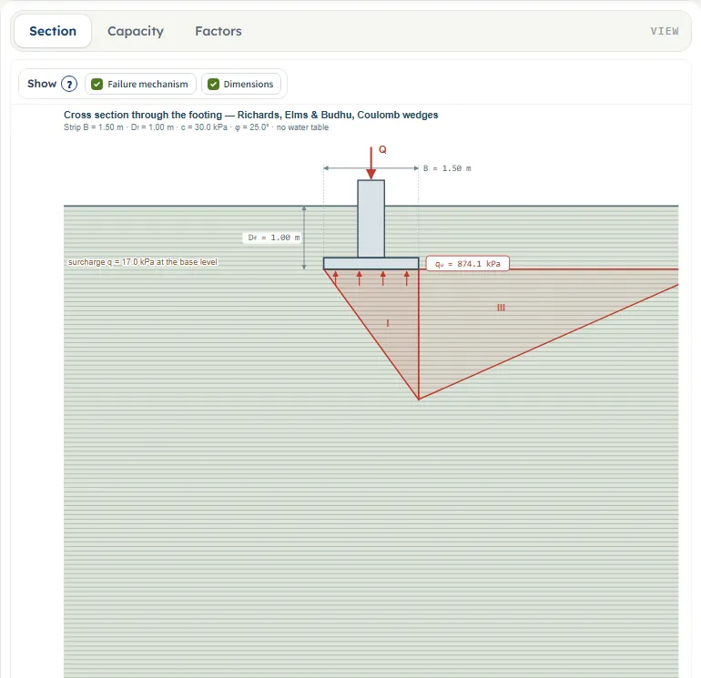
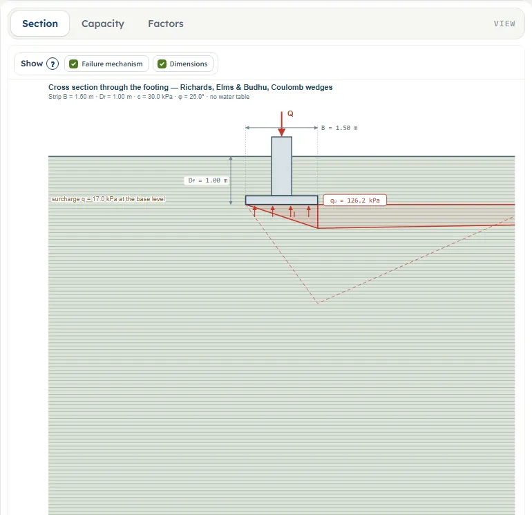
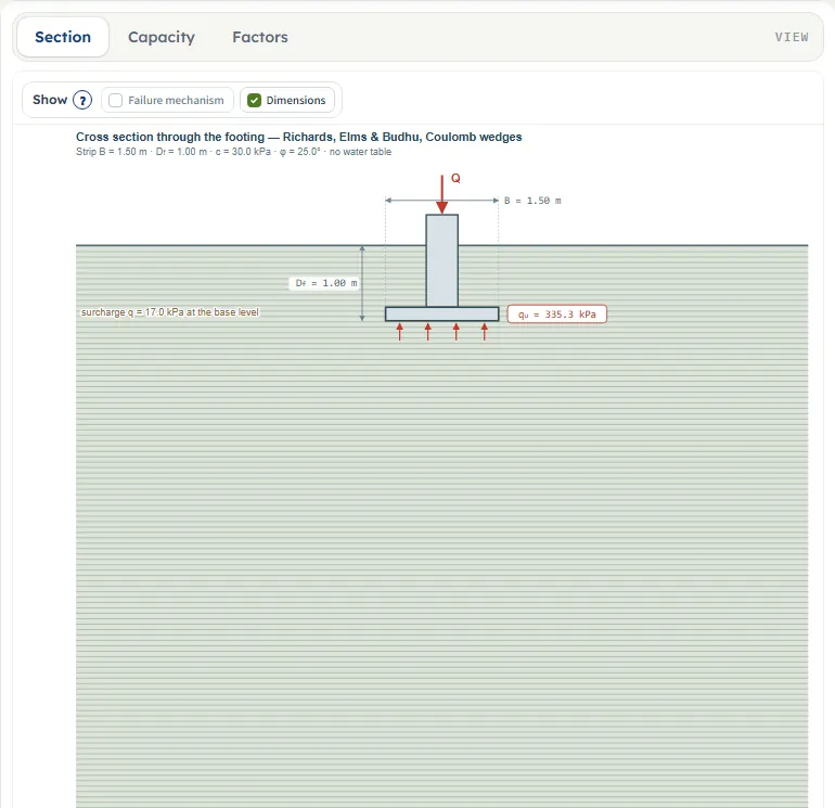
Section is a cross-section through the footing, drawn to scale for the friction angle you enter: the footing and the column with the load Q, the ground surface, the depth Df and the width B as dimensions, as dimensions. It is drawn as soon as the numbers are valid, before Analyze. After Analyze it adds the capacity qu (the seismic one when kh > 0) in a box at the base, the upward arrows, and the surcharge q = γ Df written at the base level.
The failure mechanism is the pair of wedges of the theory:
- Wedge I (ABC) is the active wedge under the footing; its slip plane AC rises at the angle αA from the horizontal. Its depth under the base is B tan αA.
- Wedge III (BCD) is the passive wedge beside the footing; its plane CD is at the angle αP. The two wedges meet on the vertical face BC, where the wall friction δ = φ/2 acts.
- With kh > 0 the earthquake wedges are drawn solid and the static wedges stay dashed, so you see how the mechanism shrinks. The note under the drawing gives the angles and, on the second line, θ = tan⁻¹[kh/(1 − kv)].
For the default example the angles are αA = 53.97° and αP = 23.85° (static), αAE = 36.21° and αPE = 6.26° (earthquake). The active wedge is then B tan αAE = 1.10 m deep instead of 2.06 m.
The Show chips
Above the section a Show bar has two chips, both on by default. Failure mechanism shows or hides the wedges (with them hidden, a note says so); Dimensions shows or hides the dimension lines. Pointing at the (?) beside Show gives a short tooltip. The chips belong to the Section view only.

Capacity: the three terms and the pressures
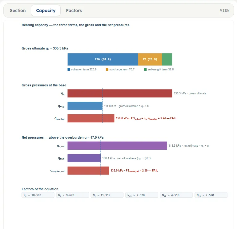
Capacity shows quE as one bar made of its three terms, the cohesion term c NcE, the surcharge term q NqE and the self-weight term ½ γ B NγE, each with its value in the legend and, where the segment is wide enough, its share in the bar. Below it the gross pressures (quE and qall,g ) and the net pressures (qu,net and qall,n ) are bars on a common scale. When you enter qapplied, a bar for it appears in each group with the actual factor of safety and PASS or FAIL, and a dashed line marks the allowable value. At the foot the six factors are listed: Nc, Nq, Nγ (static) and NcE, NqE, NγE (earthquake).
Factors: the three factors against the friction angle
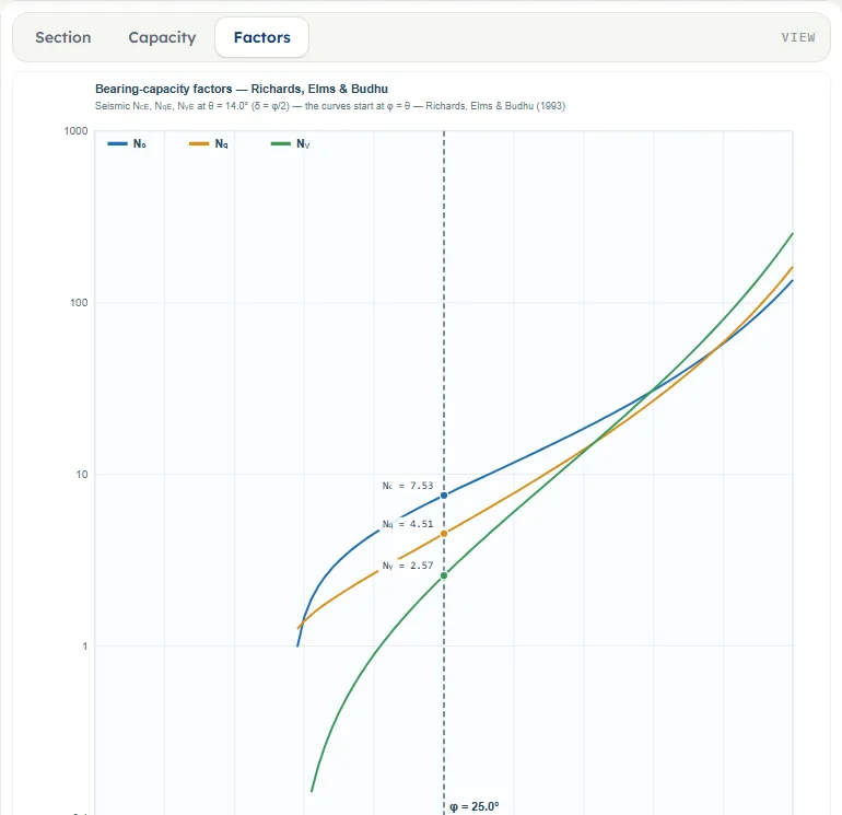
Factors plots Nc, Nq and Nγ against φ from 0° to 50° on a logarithmic scale and marks your φ with a dashed line and the three values. With kh = 0 the curves are the static factors; with kh > 0 they are the seismic NcE, NqE and NγE at your θ, and the curves start at φ = θ, where the wedges close. The note says which of the two you are looking at. For the default example the marks read NcE = 7.53, NqE = 4.51 and NγE = 2.57.
Nothing to drag, zoom or pan
The drawing has no drag handles and no zoom: change the values in the Model tab and the drawing follows. After Analyze the inputs are locked until you press Edit inputs, which clears the results; the unit system can still be changed. The drawings stay in SI (m · kPa) when you choose another unit system, and a note under them says so.
Model data: keep, save and reset
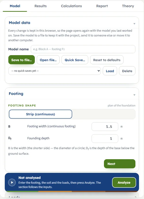
The Model data section at the top of the Model tab says that every change is kept in this browser. It holds a Model name, Save to file… and Open file… for a file you keep with the project or send on, Quick Save… with a list to Load or Delete a saved state, and Reset to defaults. When you reload the page the module reopens with your values, the unit system and, if you had analysed, the results.
Entering the model, section by section
The Model tab has, after Model data, five sections. Each opens when you click its title; Next and Back at the foot walk you through them. The tables list every field with its symbol, the unit in each unit system and its default. Where a unit is shown more than once, such as m · ft, the units are those of SI · kN, SI · tf and US in turn. A value outside the range, or a blank box, stops the analysis with a message that names it (see Messages).
Footing
The shape selector holds one option, Strip (continuous), under the label “plan of the foundation”. A note under the fields says that B is the width and Df the depth of the base below the ground surface.
| Field | Default | What to enter |
|---|---|---|
| Footing width (continuous footing) B · m · ft | 1.5 | Width of the strip. At least 0.05 m. |
| Founding depth Df · m · ft | 1 | Depth of the base below the ground surface. Zero or more; zero gives q = 0 and the surcharge term vanishes. |
Soil
One soil below the footing, as the note says: “One soil below the footing, characterised by c, φ and γ.” No water table is asked for: the module takes none in the failure zone, and the soil above the base acts as the surcharge q = γ Df only.
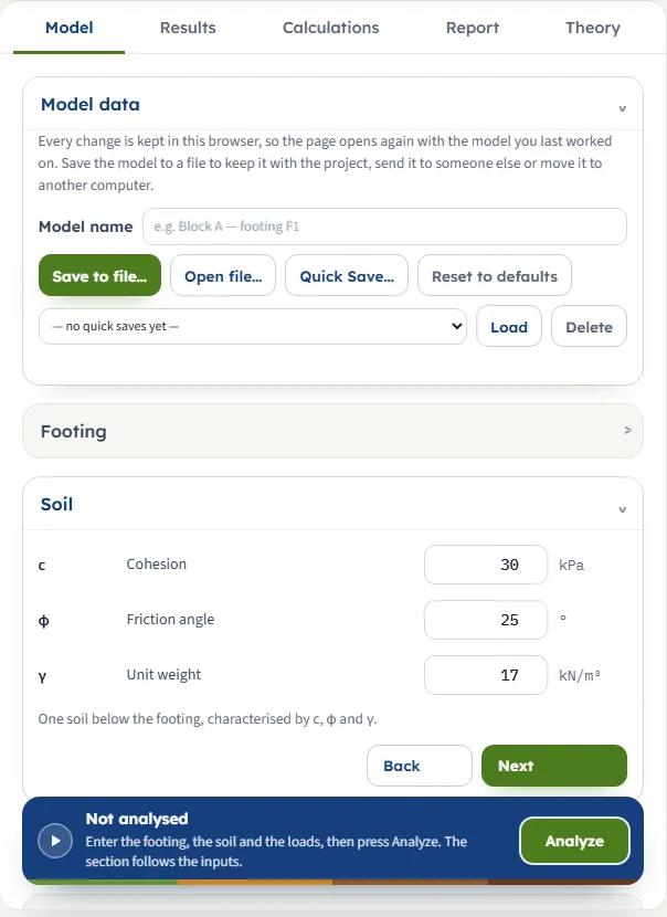
| Field | Default | What to enter |
|---|---|---|
| Cohesion c · kPa · kg/cm² · psf | 30 | Zero or more. In SI · tf the box is in kg/cm², and 30 kPa reads 0.305915. |
| Friction angle φ · ° | 25 | From 0° to 50°, and above zero for the analysis to run. |
| Unit weight γ · kN/m³ · t/m³ · pcf | 17 | At least 0.1 kN/m³. |
Loads
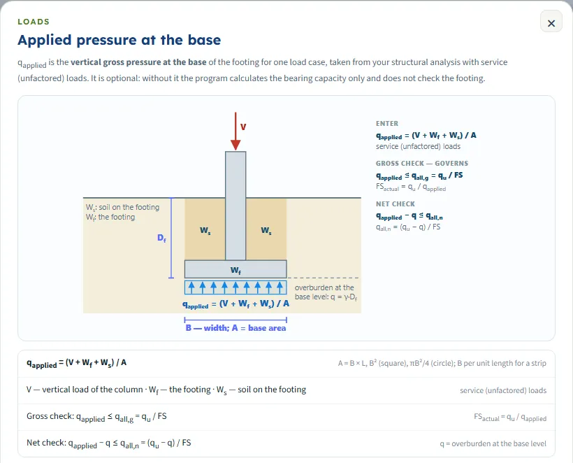
One optional field under the heading Applied load, “one load case at the base — service loads”. Leave it blank and the module reports the capacity and says the footing is not checked; enter a value and the module compares it with the allowable pressures. The (?) beside the heading opens a window with a sketch of qapplied = (V + Wf + Ws) / A and of the gross and net checks.
| Field | Default | What to enter |
|---|---|---|
| Applied vertical gross pressure at the base (optional) (optional) qapplied · kPa · t/m² · ksf | blank | The vertical gross pressure at the base, V/A, from service loads. Zero or more. |
Analysis Settings
| Field | Default | What to enter |
|---|---|---|
| Factor of safety FS · — | 3 | At least 1. It divides the capacity for the allowable pressures. |
Earthquake
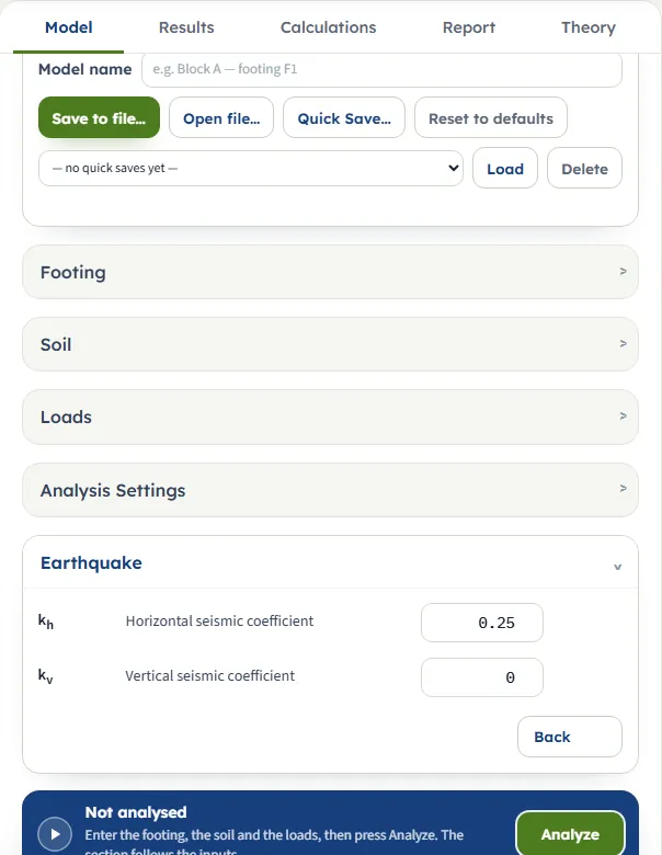
The two coefficients of the pseudo-static earthquake. Together they give θ = tan⁻¹[kh / (1 − kv)], the tilt of the resultant of the weight and the inertia; the module shows θ in the working and under the drawing.
| Field | Default | What to enter |
|---|---|---|
| Horizontal seismic coefficient kh · — | 0.25 | From 0 to 0.8. Zero gives the static case: the seismic factors equal the static ones. |
| Vertical seismic coefficient kv · — | 0 | From 0 to 0.5. A larger kv makes θ larger at the same kh. |
Units
SI · kN uses m, kPa and kN/m³. SI · tf uses m, t/m² for pressures, t/m³ for unit weight, kg/cm² for the cohesion box, and tf/m for the load. US uses ft, psf for the cohesion, pcf for the unit weight, ksf for pressures and kip/ft for the load. Values you typed are converted when you switch, and the boxes may then show unrounded numbers such as 4.92126 ft for a 1.5 m width.
Static and seismic factors: what changes
There is no method to choose in this module: the theory is fixed and so are its assumptions. What you control is how strong the earthquake is, and the module shows both sides of it.
- Factors: Nc, Nq, Nγ (static) and NcE, NqE, NγE (earthquake).
- Coefficients of the wedges: KA, KP (Coulomb) and KAE, KPE (Mononobe–Okabe, at θ).
- Wedge angles: αA, αP and αAE, αPE, with α = φ − θ in place of φ.
- Capacity: qu is reported beside the answer; quE is the value the allowable pressures and the check are built on.
The factors follow from the wedges: Nq = KP / KA, Nγ = tan αA (KP / KA − 1) and Nc = (Nq − 1) cot φ, and the seismic factors have the same forms with the earthquake quantities. The earthquake takes from the three terms very different amounts. For the default example the factors fall from Nc = 18.59, Nq = 9.67, Nγ = 11.92 to NcE = 7.53, NqE = 4.51, NγE = 2.57, that is to 0.405, 0.466 and 0.216 of the static values: the self-weight term loses most.
Analyze and read the results
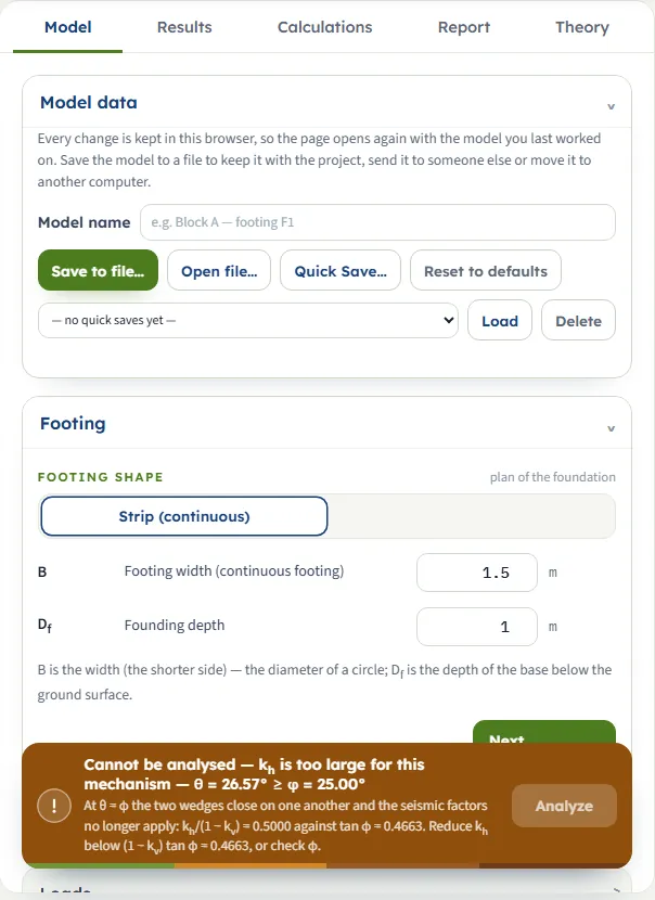
Press Analyze. If an input is missing or out of range, a window titled Cannot analyse lists what to correct. If the mechanism cannot be worked out (for example kh too large) the bar above the Analyze button turns amber and says why, and the button is greyed. Otherwise the bar reads Analysed, the inputs lock, and a window shows the warnings (if there are any). The module stays on the Model tab; open Results. Edit inputs in the bar clears the results and unlocks the inputs; Warnings reopens the window.
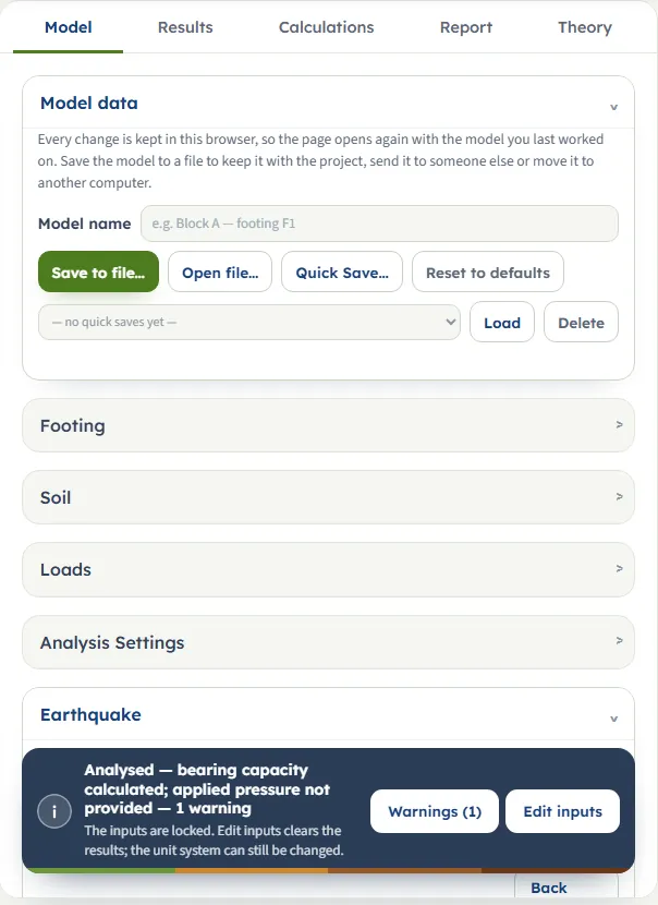
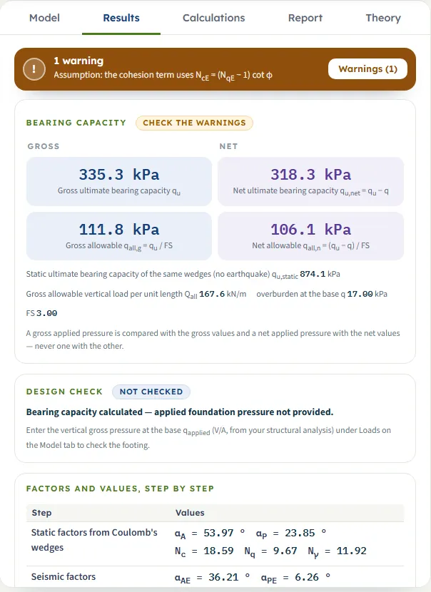
On the Results tab and in the drawings the seismic capacity is labelled qu and the static one qu,static ; the working calls the seismic one quE.
The Results tab, from the top:
- A banner with the number of warnings and the first one.
- Bearing capacity, with four large cards in two columns: Gross quE and qall,g = quE / FS, and Net qu,net = quE − q and qall,n = (quE − q) / FS. Below them the static capacity qu,static , the gross allowable load per metre of footing Qall = qall,g × B, the overburden q and FS. A note says that a gross applied pressure is compared with the gross values and a net one with the net values, never one with the other.
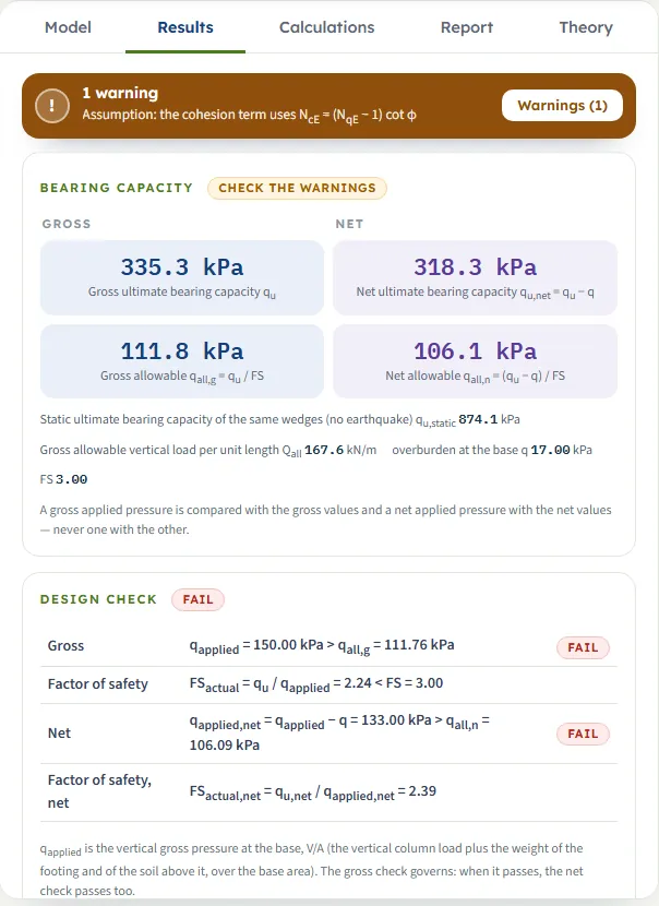
- Design check. NOT CHECKED when qapplied is blank; otherwise PASS or FAIL with a row for the gross check, the actual factor of safety FSactual = quE / qapplied, the net check and its factor of safety. The gross check governs: when it passes, the net check passes too.
- Factors and values, step by step, a table with the wedge angles and factors of each step: static, seismic, the surcharge, the two capacities, the allowable pressures and Qall.
- Contribution of each term (seismic): the cohesion, surcharge and self-weight terms, each in pressure and as a percentage of quE.
- Warnings, repeated at the foot.
Gross and net
The gross pressures are the total pressure at the base; the net pressures are what the footing adds to the overburden q that already acted there. They are two conventions for applying the factor of safety, not conversions of one another: the gross convention divides the whole capacity by FS, the net convention only the part above q, so qall,n + q is larger than qall,g and the gross convention is the stricter. For the default example qall,g = 111.76 kPa and qall,n = 106.09 kPa. State which convention your design follows.
Calculations, Report and Theory
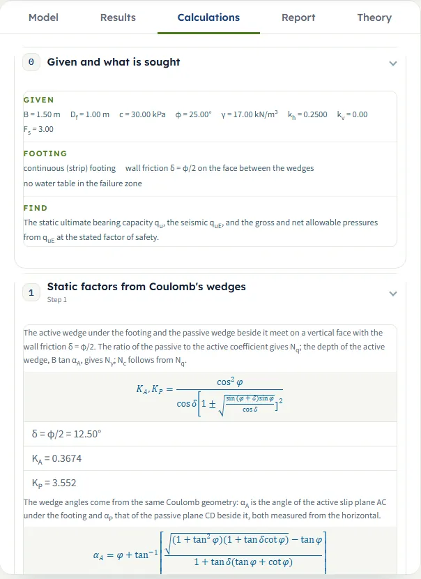
The Calculations tab writes the working in steps, each with its formula, your numbers and the result:
- Given and what is sought: your inputs, the footing assumptions and what is found.
- Static factors from Coulomb’s wedges: δ = φ/2, KA, KP, the wedge angles αA, αP with the depth B tan αA, and Nq, Nγ, Nc.
- Seismic factors: θ, KAE, KPE, α = φ − θ, αAE, αPE, the depth B tan αAE, the factors NqE, NγE, NcE and their ratios to the static ones. With kh = 0 the step says that the seismic factors equal the static ones.
- Surcharge at the base level: q = γ Df.
- Static ultimate bearing capacity: qu term by term.
- Seismic ultimate bearing capacity: quE term by term, with the contribution table. From here on qu in the working stands for quE.
- Apply the factor of safety: qu,net , qall,g , qall,n .
- Compute the gross allowable load: Qall.
- Check the applied foundation pressure: the PASS or FAIL rows, or the statement that no pressure is entered.
Then come the warnings and the Answer sentence. The equations are typeset, and the same text is the calculation part of the report.
Report
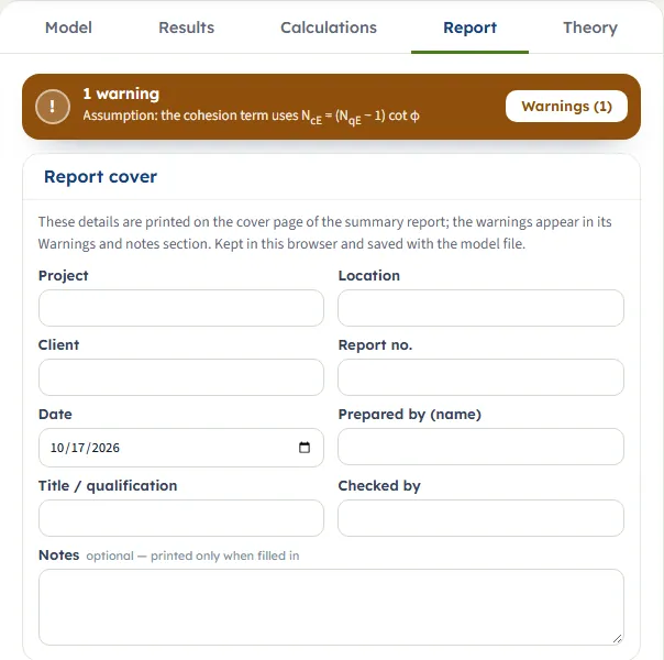
The Report tab has a Report cover form (Project, Location, Client, Report no., Date, Prepared by, Title / qualification, Checked by and optional Notes), which is kept in the browser and saved with the model file, and two buttons: Save as PDF (the report opens in a print window; choose Save as PDF there) and Download Word (.docx). Both are available once the model is analysed; below them a preview shows the report. It has seven parts: introduction and scope, input data (with the section drawing), the calculation, results (with the capacity drawing), warnings and notes, a summary and references.
Theory
The Theory tab derives the method in ten sections: Scope and assumptions; The static failure surface; The surcharge term; The self-weight term; The static bearing capacity; Earthquake loading; How much the earthquake takes away; Allowable pressure and the check; Worked example (computed live from the module’s opening model); and References. Open all and Close all expand or fold the sections. Its figures are drawn to scale from the equations.
Worked example
The opening model: a strip footing B = 1.5 m at Df = 1 m on soil with c = 30 kPa, φ = 25°, γ = 17 kN/m³, in an earthquake with kh = 0.25 and kv = 0, with FS = 3. Each number below is on the screen when you run the module.
| Step | Result |
|---|---|
| Static wedges, δ = φ/2 = 12.50° | KA = 0.3674, KP = 3.552; αA = 53.97°, αP = 23.85° |
| Static factors | Nq = KP/KA = 9.67, Nγ = 11.92, Nc = 18.59 |
| Earthquake angle | θ = tan⁻¹ 0.25 = 14.04°; α = φ − θ = 10.96° |
| Seismic wedges | KAE = 0.6006, KPE = 2.709; αAE = 36.21°, αPE = 6.26°; the active wedge is 1.10 m deep (2.06 m static) |
| Seismic factors | NqE = 4.510, NγE = 2.570, NcE = 7.528 |
| Surcharge | q = 17 × 1.00 = 17.00 kPa |
| Static capacity | qu = 557.79 + 164.39 + 151.96 = 874.14 kPa |
| Seismic capacity | quE = 30 × 7.528 + 17 × 4.510 + ½ × 17 × 1.5 × 2.570 = 225.83 + 76.67 + 32.77 = 335.28 kPa |
| Net and allowable | qu,net = 318.28 kPa; qall,g = 111.76 kPa; qall,n = 106.09 kPa |
| Allowable load | Qall = 111.76 × 1.5 = 167.64 kN/m |
The earthquake leaves 38 % of the static capacity. With no applied pressure the design check reads NOT CHECKED. Enter qapplied = 100 kPa and it reads PASS: FSactual = 335.28 / 100 = 3.35, against 3.00; the net pressure 83.00 kPa is below qall,n = 106.09 kPa, with FSactual,net = 3.83. With qapplied = 150 kPa it reads FAIL: FSactual = 2.24, and the net factor 2.39. With kh = 0 and qapplied = 200 kPa the same footing passes, with FSactual = 4.37.
The same example in other units
Switch to US and the example reads B = 4.92126 ft, Df = 3.28084 ft, c = 626.563 psf and γ = 108.22 pcf; the module gives quE = 7.002 ksf, qu,static = 18.26 ksf, qall,g = 2.334 ksf, qall,n = 2.216 ksf and Qall = 11.49 kip/ft. Switch to SI · tf and it gives quE = 34.19 t/m², qu,static = 89.14 t/m² and Qall = 17.09 tf/m. Each equals the SI · kN answer, converted: 335.28 kPa / 47.88 = 7.002 ksf and 335.28 kPa / 9.807 = 34.19 t/m².
How each input changes the answer
Each row is a run of the module that changes one input from the default example (B = 1.5 m, Df = 1 m, c = 30 kPa, φ = 25°, γ = 17 kN/m³, kh = 0.25, kv = 0, FS = 3). Pressures are in kPa; “Share” is quE as a fraction of the static qu of the same soil.
The earthquake coefficient
| kh (θ) | NcE · NqE · NγE | quE | Share |
|---|---|---|---|
| 0 (0°, static) | 18.59 · 9.67 · 11.92 | 874.1 | 100 % |
| 0.1 (5.71°) | 13.54 · 7.31 · 7.01 | 620.0 | 71 % |
| 0.2 (11.31°) | 9.36 · 5.36 · 3.74 | 419.6 | 48 % |
| 0.25 (14.04°), default | 7.53 · 4.51 · 2.57 | 335.3 | 38 % |
| 0.3 (16.70°) | 5.84 · 3.72 · 1.65 | 259.5 | 30 % |
| 0.4 (21.80°) | 2.74 · 2.28 · 0.4230 | 126.2 | 14 % |
| 0.45 (24.23°) | 1.07 · 1.50 · 0.0735 | 58.68 | 7 % |
The static capacity is qu = 874.1 kPa in every row. The capacity falls steadily and then steeply as θ approaches φ = 25°: at kh = 0.4 it is 14 % of the static value and at 0.45 it is 7 %. At kh = 0.4 and 0.45 the module warns that the mechanism is near its limit. At kh = 0.5 it stops, because θ = 26.57° is not below φ.
The other inputs
| Change | quE | qall,g |
|---|---|---|
| Default | 335.3 | 111.8 |
| kv = 0.2 | 241.7 | 80.58 |
| c = 0 | 109.4 | 36.48 |
| c = 60 kPa | 561.1 | 187.0 |
| φ = 20° | 191.9 | 63.98 |
| φ = 30° | 559.9 | 186.6 |
| B = 3 m | 368.0 | 122.7 |
| Df = 0 | 258.6 | 86.20 |
| Df = 2 m | 411.9 | 137.3 |
| γ = 19 kN/m³ | 348.2 | 116.1 |
| FS = 2 | 335.3 | 167.6 |
- kv. Raising kv from 0 to 0.2 at kh = 0.25 raises θ from 14.04° to 17.35°, takes the factors to 5.44 · 3.54 · 1.45 and lowers quE from 335.3 to 241.7 kPa.
- Cohesion. The cohesion term is linear in c: c = 0 gives 109.4 kPa (static 316.4), c = 60 kPa gives 561.1 kPa. The factors do not change.
- Friction angle. φ changes the factors and the room before the wedges close. At φ = 20° the same kh = 0.25 gives θ/φ = 0.70, the factors 4.52 · 2.65 · 0.8925 and quE = 191.9 kPa; at 30° it gives the factors 11.70 · 7.76 · 6.03 and 559.9 kPa.
- Width. Only the self-weight term depends on B: doubling it from 1.5 to 3 m raises quE from 335.3 to 368.0 kPa, while the allowable load Qall rises from 167.64 to 368.0 kN/m.
- Depth. Df acts through q = γ Df. At Df = 0, q = 0, the surcharge term vanishes and the net and gross values are equal (258.6 kPa); at 2 m quE is 411.9 kPa.
- Unit weight. γ acts through the surcharge and self-weight terms: 19 kN/m³ gives 348.2 kPa.
- Factor of safety. FS does not change quE; at FS = 2 the allowable pressure is 167.6 kPa instead of 111.8 kPa.
Messages: stops, cautions and notes
Messages are shown in three places: a window titled Cannot analyse when a field is wrong, an amber bar above the Analyze button when the mechanism cannot be worked out, and the Warnings window with the banner on the results tabs.
| Kind | When | What the module says |
|---|---|---|
| Stop | φ = 0 | The amber bar reads “Cannot be analysed — φ = 0.00°: the theory needs a friction angle”, and below it: “The method builds the capacity from Coulomb wedges in a frictional soil. Enter φ > 0, or use Terzaghi or Meyerhof for undrained clay.” |
| Stop | θ is not below φ | The amber bar reads “Cannot be analysed — kh is too large for this mechanism — θ = 26.57° ≥ φ = 25.00°”, and below it: “At θ = φ the two wedges close on one another and the seismic factors no longer apply: kh/(1 − kv) = 0.5000 against tan φ = 0.4663. Reduce kh below (1 − kv) tan φ = 0.4663, or check φ.” |
| Stop | A value is out of range | The window title counts the errors (“Cannot analyse — 1 input error”, “— 2 input errors”) and each message is on its own line, in the order B, Df, c, φ, γ, kh, kv, qapplied, FS. Field errors come before the mechanism stops. For example φ = 55° with kh = 0.9 lists “Friction angle (φ) must be at most 50°.” and “Horizontal seismic coefficient (kh) must be at most 0.8.” The messages: “Friction angle (φ) must be at most 50°.”, “Horizontal seismic coefficient (kh) must be at most 0.8.”, “Vertical seismic coefficient (kv) must be at most 0.5.”, “Footing width (continuous footing) (B) must be at least 0.05 m.”, “Unit weight (γ) must be at least 0.1 kN/m³.”, “Factor of safety (FS) must be at least 1.”, “Cohesion (c) must be at least 0 kPa.”, “Founding depth (Df) must be at least 0 m.”, “Applied vertical gross pressure at the base (optional) (qapplied) must be at least 0 kPa.” |
| Stop | A required box is blank | “Footing width (continuous footing) (B) is missing.” and likewise for the other required fields, for example “Horizontal seismic coefficient (kh) is missing.” qapplied may stay blank. |
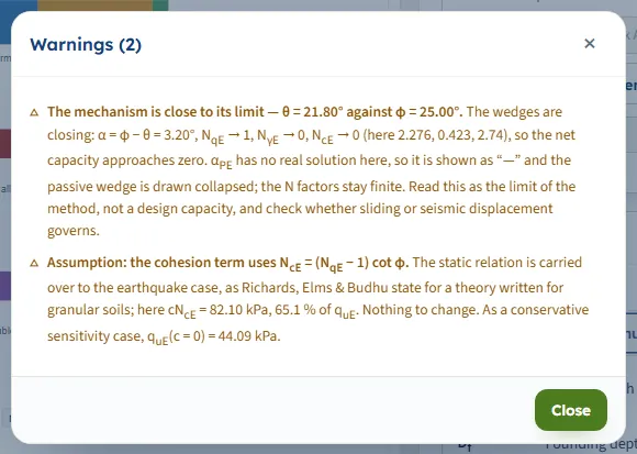
| Warning | θ is above 0.85 φ, or the passive angle has no real solution | “The mechanism is close to its limit — θ = 21.80° against φ = 25.00°.” The wedges are closing: α = φ − θ = 3.20°, NqE → 1, NγE → 0, NcE → 0, so the net capacity approaches zero. If αPE has no real solution it is shown as “—” and the passive wedge is drawn collapsed; the N factors stay finite. The module advises reading this as the limit of the method, not a design capacity, and checking whether sliding or seismic displacement governs. |
| Warning | c is above zero | “Assumption: the cohesion term uses NcE = (NqE − 1) cot φ.” It gives the share of the cohesion term in quE and the sensitivity case quE(c = 0). With c = 0 the warning does not appear. |
| Status | After Analyze | “Analysed — bearing capacity calculated; applied pressure not provided.” With a pressure entered it reads, for example, “Analysed — PASS: qapplied ≤ qall,g, FSactual = 3.35” or “Analysed — FAIL: qapplied > qall,g, FSactual = 2.24”, followed by the number of warnings. |
With kh = 0.4 the warnings window lists two entries, the caution about the limit first and then the cohesion assumption, with quE(c = 0) = 44.09 kPa.
Good practice and common mistakes
- Run the static case too. Set kh = 0 and the module gives the static capacity of the same wedges; the ratio quE / qu is the share the earthquake leaves.
- Take the check from quE. The allowable pressures and the PASS or FAIL are built on the seismic capacity. The static value is for comparison.
- Mind the limit. Near θ = φ the capacity is small and falls fast; the module marks it with a caution. Treat the number as the limit of the method, and check sliding and seismic displacement.
- Enter the gross pressure. qapplied is V/A including the footing and the soil above it, from service loads. Do not enter a net pressure; a gross pressure is compared with the gross values and a net one with the net values.
- Keep the soil one soil. The module reads one set of c, φ and γ for the zone below the base; no water table is taken in the failure zone.
- Use the right module for the rest. A clay with φ = 0, a square or circular footing, or an inclined load need the static modules of this family: Terzaghi, Meyerhof, Hansen or Vesic.
- Mind the unit of the cohesion box. In SI · tf it is kg/cm², not t/m².
- Save what you need. The model is kept in your browser, but Save to file keeps it with the project.
Frequently asked questions
What does the Seismic bearing capacity module calculate?
The static and the seismic ultimate bearing capacity of a strip footing on c–φ soil by the Coulomb-wedge theory of Richards, Elms and Budhu (1993), the gross and net allowable pressures from the seismic capacity, the allowable load per metre, and a PASS or FAIL check of an applied pressure. For the default example (B = 1.5 m, Df = 1 m, c = 30 kPa, φ = 25°, γ = 17 kN/m³, kh = 0.25) the seismic capacity is 335.3 kPa and the static 874.1 kPa.
What is the difference between Nc, Nq, Nγ and NcE, NqE, NγE?
The first three are the factors of the two Coulomb wedges with no earthquake; the second three are the same factors with the earthquake angle θ, worked out from the Mononobe–Okabe coefficients. For the default example they are 18.59, 9.67, 11.92 against 7.53, 4.51, 2.57. The seismic capacity quE uses the second set and is what the allowable pressures are built on.
How do I choose kh and kv?
They come from your seismic design; the module takes the values you enter, kh from 0 to 0.8 and kv from 0 to 0.5. With kv = 0 only the horizontal inertia acts, and θ = tan⁻¹ kh. Since the module draws the wedges and writes θ for every run, you can change kh and see at once what it does.
How much does an earthquake reduce the bearing capacity in the module?
For the default soil the capacity is 71 % of the static value at kh = 0.1, 48 % at 0.2, 38 % at 0.25, 30 % at 0.3 and 14 % at 0.4. The reduction grows faster as θ approaches φ, and the self-weight term falls the most.
Why does the module stop when kh is large?
The seismic factors need θ below φ. At θ = φ the two wedges close on one another, so for φ = 25° and kv = 0 the module stops at kh = 0.4663 and tells you the limit (1 − kv) tan φ. Just below it, above θ = 0.85 φ, it gives a caution that the capacity is near the limit of the method.
Is the footing checked against the static or the seismic capacity?
Against the seismic capacity quE. The gross check compares qapplied with qall,g = quE / FS, the net check compares qapplied − q with qall,n ; the static capacity is shown beside the answer for comparison. With kh = 0 the two are equal.
Can I use it for a square or circular footing, or for clay with φ = 0?
No. The module is for a continuous (strip) footing on a soil with φ > 0, and its shape selector holds one option. For φ = 0 it stops and points to Terzaghi or Meyerhof; for other footing shapes and static design use the other modules of the family.
Why is the static capacity different from the other bearing capacity modules?
The static value here is the capacity of the same two-wedge mechanism that gives the seismic one, not the classical Prandtl-type value of Terzaghi, Meyerhof, Hansen or Vesic. It is the value the seismic capacity is reduced from. For a static design, use those modules.
Does the module include the water table or a horizontal load?
No water table is taken in the failure zone, and the soil above the base acts as the surcharge q = γ Df only. The pseudo-static horizontal inertia is carried by kh, so no separate horizontal load is entered; an independent horizontal force, a moment or an eccentricity is outside this calculation, and a method with inclination factors (Meyerhof, Hansen, Vesic) is the place for the inclined load.
What is the warning about the cohesion term?
The cohesion term uses NcE = (NqE − 1) cot φ, the static relation carried over to the earthquake case. When c is above zero the module says so and gives the share of the term in quE (67.4 % for the default example) and the capacity with c = 0 (109.45 kPa). With c = 0 there is no warning.
Can I drag the wedges or zoom the drawing?
No. The drawing has no drag handles and no zoom; the Show chips switch the wedges and the dimensions on and off. Change the values in the Model tab and the drawing follows. After Analyze the inputs are locked until you press Edit inputs.
Does the module remember my inputs, and which units does it use?
Yes: every change is kept in the browser, and the page reopens on your last model, its unit system and its results. Reset to defaults brings the example back in the unit system you have chosen; Save to file and Quick Save keep copies. The units are SI · kN, SI · tf or US, switchable at any time. The default example gives 335.3 kPa, 34.19 t/m² or 7.002 ksf.