

What the module calculates
Hansen gives the ultimate and the allowable bearing capacity of a shallow footing by Hansen’s (1970) equation. It is the module of the family to use when the footing is near sloping ground, when its base is tilted from the horizontal, or when the load is inclined: besides the usual shape and depth corrections it applies Hansen’s inclination, base-tilt and ground-slope factors, and Hansen’s own bearing capacity factor Nγ.
The three terms are the cohesion term, the surcharge term (the weight of the soil above the base, q) and the self-weight term. Nc, Nq and Nγ depend on the friction angle φ alone; s are the shape factors, d the depth factors, i the inclination factors, b the base-tilt factors and g the ground-slope factors. For a level base on level ground under a vertical load the last three sets are all 1. At φ = 0 the cohesion term takes Hansen’s additive form, which the Calculations tab writes out.
What you can describe
- A strip, square, rectangular or circular footing: width B (the diameter of a circle), length L of a rectangle, and the founding depth Df.
- One soil below the footing: cohesion c, friction angle φ and unit weight γ, with an optional water table (saturated unit weight and depth Dw).
- A base tilt η and a ground slope ω (both in degrees).
- The load as one load case: the horizontal pressure h = H/A and, optionally, the vertical gross pressure qapplied = V/A at the base.
- The factor of safety FS.
The module gives the gross and the net ultimate bearing capacity qu and qu,net , the gross and the net allowable pressures qall,g and qall,n , the gross allowable load Qall, all the factors with their values, the working step by step, a drawing of the failure mechanism to scale and a report as a PDF or a Word file. When you also enter qapplied it checks the footing and shows PASS or FAIL.
Which module of the family for which case
- A vertical or inclined load on level ground, with shape, depth and inclination factors: Meyerhof.
- The classical equation, with general and local shear: Terzaghi.
- The same corrections as in this module, with Vesic’s factors: Vesic.
- A strip footing in an earthquake: Seismic bearing capacity.
- The family page lists the five modules.
Before you start: what you need
Have these ready from your design and your soil data:
| What | Notes |
|---|---|
| The footing From: your design | Shape, width B (the shorter side), length L for a rectangle, and the depth Df of the base below the ground surface. |
| The soil From: your investigation | Cohesion c, friction angle φ (0 to 50°) and unit weight γ of the soil below the footing. Use effective-stress parameters for a drained case and undrained cohesion with φ = 0 for a clay under short-term loading. |
| The water table From: the borehole logs | Its depth Dw below the ground surface and the saturated unit weight γsat, when water is within reach of the footing. |
| Base tilt and ground slope From: your layout | η, the tilt of the base from the horizontal, and ω, the slope of the ground next to the footing, both in degrees (0 to 45°). Leave both at 0 for a level base on level ground. |
| The load of the case From: your structural analysis | The horizontal pressure h = H/A and the vertical gross pressure qapplied = V/A at the base, with service (unfactored) loads: the column load plus the weight of the footing and of the soil on it, over the base area. Needed for the check, and needed whenever h is above zero. |
| The factor of safety From: your design rules | FS, at least 1. |
Quick start in seven steps
- Open the module and choose the units
Open Hansen from the Bearing Capacity family. Pick SI · kN, SI · tf or US in the header; you can change it at any time.
- Describe the footing
In Footing choose Strip, Square, Rectangular or Circular and type B (and L for a rectangle) and Df.
- Enter the soil and the water
In Soil type c, φ and γ. In Groundwater choose Present or None; with water, type γsat and Dw.
- Enter the tilt, the slope and the load
In Base tilt and ground slope type η and ω. In Loads type h and, for the check, qapplied. In Analysis Settings type FS.
- Press Analyze
Press Analyze at the foot of the Model tab. The bar reads Analysed with the verdict when qapplied is entered, and the inputs lock.
- Read the answer
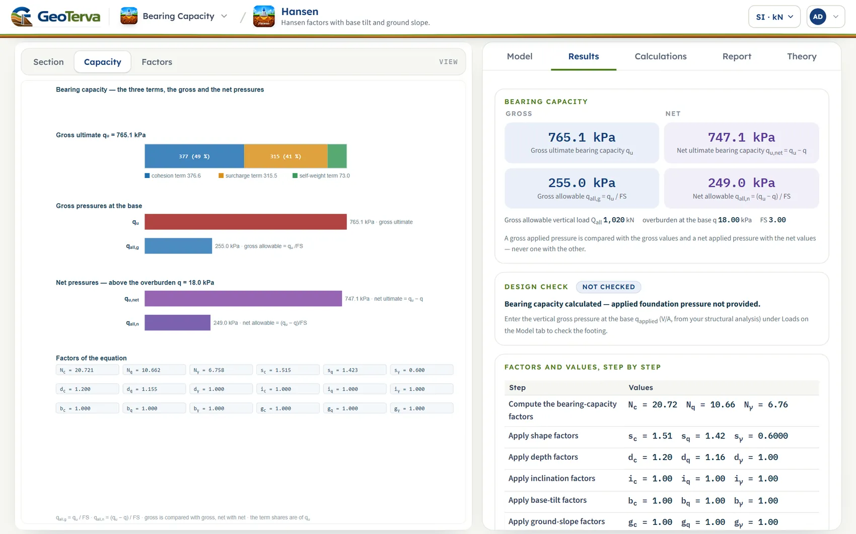
The Results tab gives the gross and net ultimate bearing capacity, the gross and net allowable pressures and the check. The Capacity and Factors views draw them.
- Take the working and the report
The Calculations tab writes out the steps with your numbers. The Report tab saves a PDF or a Word file.
The screen: section, capacity and factors
The layout is the one every GeoTerva module shares, described in the workspace guide: the drawing on the left, the tabs on the right. The drawing has three views, chosen with the buttons above it:
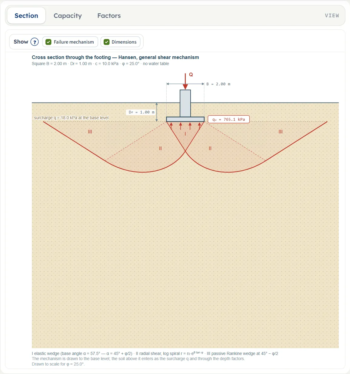
- Section is a cross section through the footing in the ground, drawn to scale: the footing, the depth Df, the width B, the surcharge q at the base level and, after Analyze, qu under the base. It shows the general shear mechanism of the method for your φ: the elastic wedge under the base (I), the radial shear zone (II) and the passive wedge (III). It follows the inputs as you type.
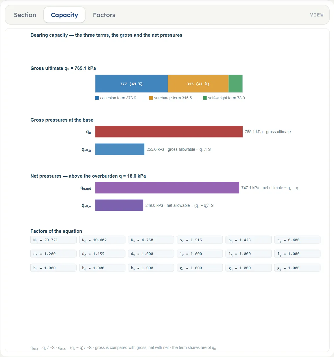
- Capacity is the answer drawn: a bar split into the cohesion, surcharge and self-weight terms; the gross pressures qu and qall,g ; the net pressures qu,net and qall,n ; and the factors of the equation. Before Analyze it says “Press Analyze”.
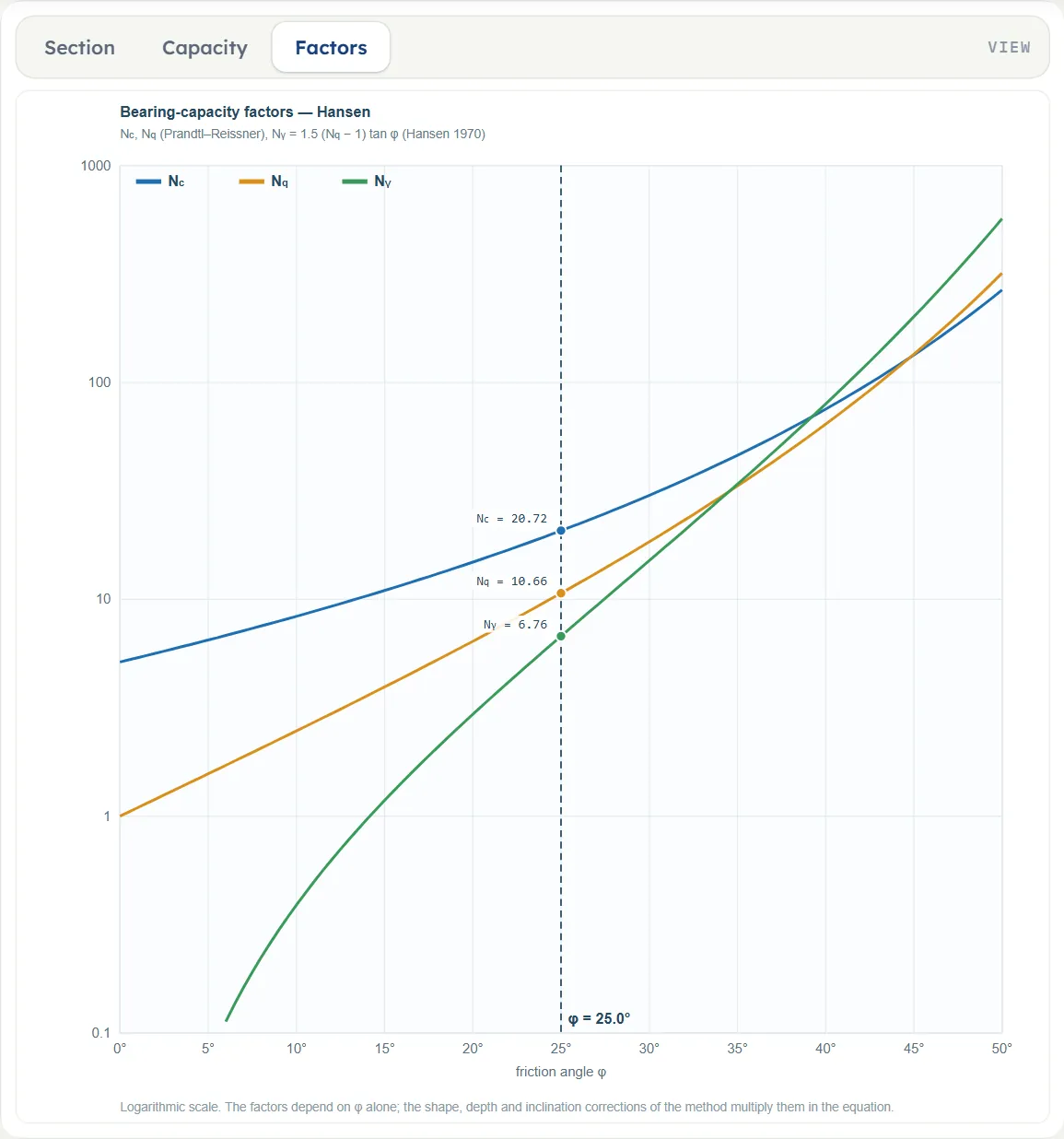
- Factors plots Nc, Nq and Nγ against φ (logarithmic scale), with the values at your φ marked.
The Show chips
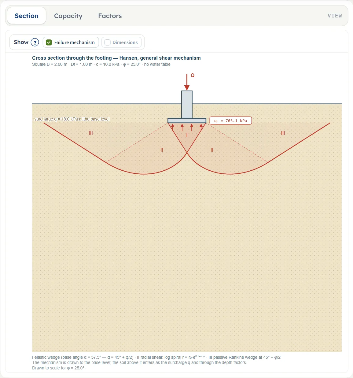
Above the Section, a bar holds two chips, both checked by default. Failure mechanism draws the three zones of the mechanism, and Dimensions draws the dimension lines of B and Df. The Capacity and Factors views have no chips.
Dragging and zoom
The drawings are set by the numbers: nothing on them can be dragged and they have no zoom buttons. Change the inputs on the Model tab and the Section follows.
The angles and the load on the drawing
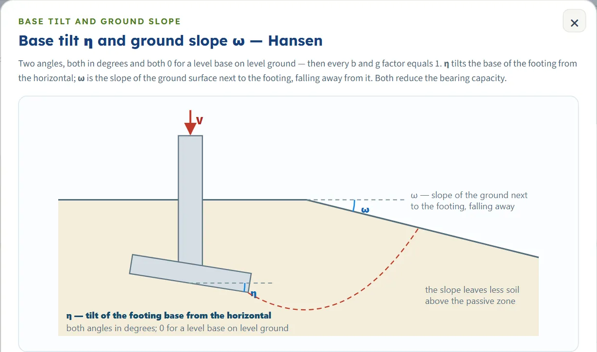
The Section draws the angles you enter. With η above 0 a dashed ray marks the base tilt (“base tilt η = …°”); with ω above 0 the ground slope is drawn and labelled “ground slope ω = …°”; and when h and qapplied are entered the load arrow reads “Q inclined …° from vertical”, the angle being arctan(h/qapplied), even before Analyze. When the sloping ground drops below the base level inside the mechanism the drawing says “Caution: the sloping ground drops below the base level inside the mechanism; the part of the mechanism above the ground is not drawn.” The factors that follow from the angles are listed on the Capacity view, on the Results tab and in the Calculations. The (?) window of the Base tilt and ground slope section draws the two angles, see below.
Entering the model, section by section
The Model tab has seven sections: Model data, Footing, Soil, Groundwater, Base tilt and ground slope, Loads and Analysis Settings. Each opens when you click its title, and opening one closes the one that was open; Next and Back walk you through them, and Analyze waits below the last one. In the tables, a unit shown three times gives the units of SI · kN, SI · tf and US in turn. Defaults are shown in SI; in the other systems the boxes show the converted values, for example 6.56168 ft for B = 2 m, 208.854 psf for c = 10 kPa or 114.586 pcf for γ = 18 kN/m³.
Model data
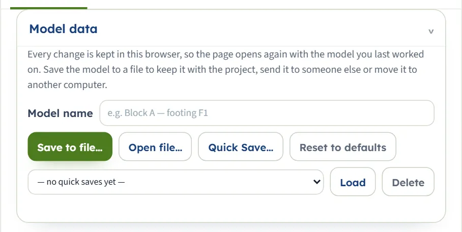
The first section holds the model name, Save to file…, Open file…, Quick Save… with its list and Load and Delete, and Reset to defaults. It works as described in the workspace guide. The list reads “— no quick saves yet —” until you save a version.
Footing
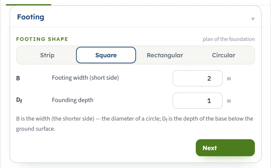
Choose the shape with the four buttons; the Square is selected at the start. The footing takes its dimensions from B and Df, and L appears for a rectangle. The shape sets the ratio B/L of the shape factors: 0 for a strip, 1 for a square and for a circle (whose B is the diameter) and B/L for a rectangle.
| Field | Unit | Default |
|---|---|---|
| Footing width (short side) B The width, the shorter side; the diameter of a circle. At least 0.05 m. | m · ft | 2 |
| Footing length (long side) L At least 0.05 m, and not shorter than B. Shown when the shape is Rectangular. | m · ft | 2 |
| Founding depth Df The depth of the base below the ground surface. Zero or more. | m · ft | 1 |
Soil
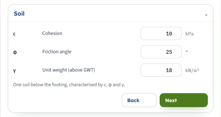
One soil below the footing, described by c, φ and γ. For layered ground enter the values of the layer that governs under the footing, the weaker one for a conservative result.
| Field | Unit | Default |
|---|---|---|
| Cohesion c Zero or more. | kPa · kg/cm² · psf | 10 |
| Friction angle φ From 0 to 50°. At 0 the cohesion term takes the additive form of the undrained case. | ° | 25 |
| Unit weight (above GWT) γ The unit weight of the soil above the water table. At least 0.1 kN/m³. | kN/m³ · t/m³ · pcf | 18 |
Groundwater
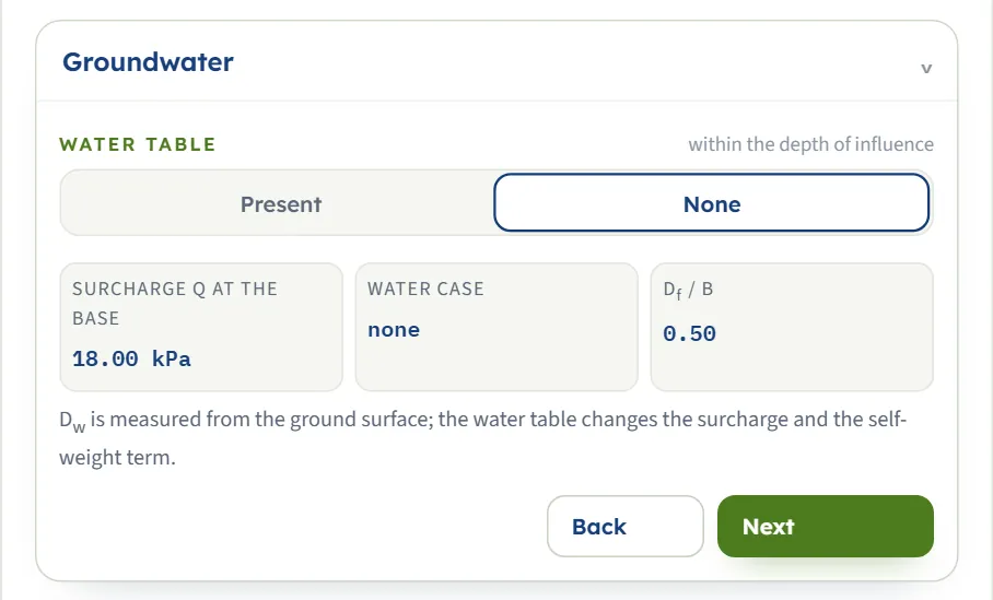
Choose Present or None. With a water table the saturated unit weight and the depth Dw are asked for. Three small read-outs follow your inputs: the surcharge q at the base, the water case, and Df/B. The cases are the ones the Calculations tab names: the water table above the base, at or within one width below it (the self-weight term then uses a weighted unit weight), or deeper than one width below it (no effect).
| Field | Unit | Default |
|---|---|---|
| Water table: Present or None None means no water table within the depth of influence. | — | None |
| Saturated unit weight γsat The unit weight below the water table. Shown when the water table is Present. | kN/m³ · t/m³ · pcf | 19 |
| Water table depth Dw Measured from the ground surface. Zero or more. Shown when the water table is Present. | m · ft | 3 |
Base tilt and ground slope
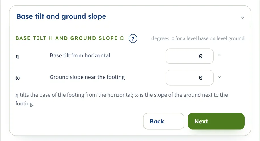
The two angles that distinguish Hansen’s equation. η tilts the base of the footing from the horizontal; ω is the slope of the ground next to the footing, falling away from it. Both reduce the capacity; with both at 0 every b and g factor is 1. The (?) beside the heading opens a window with a drawing of the two angles and the formulas.
| Field | Unit | Default |
|---|---|---|
| Base tilt from horizontal η From 0 to 45°. | ° | 0 |
| Ground slope near the footing ω From 0 to 45°; for φ above 0 it may not exceed φ. | ° | 0 |
Loads
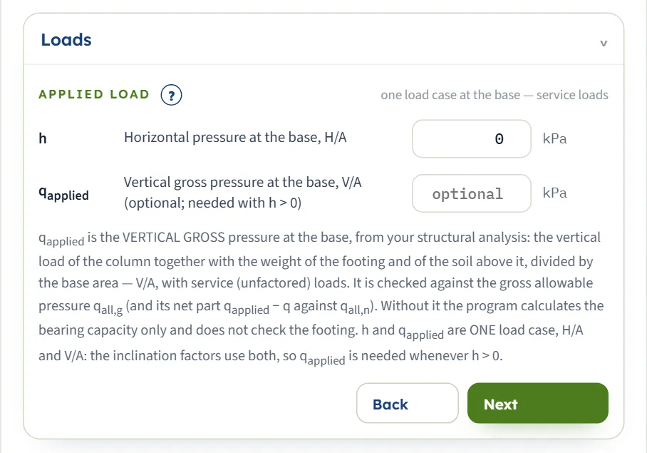
The load is one load case: the horizontal pressure h = H/A and the vertical gross pressure qapplied = V/A at the base, with service loads. The inclination factors use both, so qapplied is needed whenever h is above 0. Without qapplied the module gives the bearing capacity and the check reads NOT CHECKED. The (?) opens a window with a drawing of the load case, the gross and the net check.
| Field | Unit | Default |
|---|---|---|
| Horizontal pressure at the base, H/A h Zero or more. | kPa · t/m² · ksf | 0 |
| Vertical gross pressure at the base, V/A qapplied Optional; needed with h above 0 and for the check. Zero or more. | kPa · t/m² · ksf | empty |
Analysis Settings
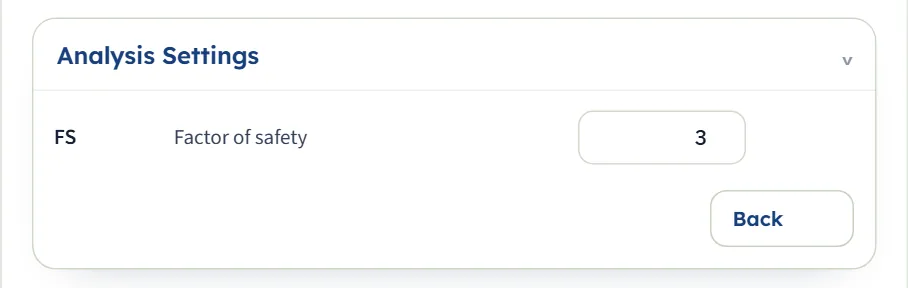
The factor of safety divides the ultimate capacity into the allowable pressures.
| Field | Unit | Default |
|---|---|---|
| Factor of safety FS At least 1. | — | 3 |
Choosing the shape, the water and the load case
The module has one method, Hansen’s; what you choose is the description of the footing and of the case.
| Choice | What it does |
|---|---|
| Shape | Sets B/L in the shape factors sc = 1 + (B/L)(Nq/Nc), sq = 1 + (B/L) sin φ, sγ = 1 − 0.4(B/L). A strip carries no shape correction. For the example, a strip gives qu = 592.0 kPa, a 2 × 4 m rectangle 678.5 kPa and a square 765.1 kPa; a circle of the same B gives the same as the square. |
| Water table | Changes the surcharge q and the self-weight term. A table above the base gives q = 13.6 kPa (against 18.0) at Dw = 0.5 m; one at the base roughly halves the self-weight term; one deeper than one width below the base changes nothing. |
| Horizontal load h | Reduces every term through the inclination factors. It needs qapplied, and it must stay below qapplied + c cot φ (below c when φ = 0). |
| Tilt η and slope ω | Reduce the capacity through the b and g factors. ω may not exceed φ. |
Which should I pick?
- Hansen’s equation when the footing is at the top of a slope or an embankment, when the base is sloped, or when the horizontal load is significant. For a level base and level ground under a vertical load the inclination, tilt and slope factors are 1 and the equation reduces to the shape and depth factors with Hansen’s own Nγ.
- The load case from your analysis: give h and qapplied from the same load combination, with service loads. A slope or a tilt does not need a horizontal load; a horizontal load needs qapplied.
- φ = 0 for a clay under short-term loading, with the undrained cohesion as c; Nγ is then 0 and the self-weight term vanishes.
Analyze and read the results
Press Analyze. The bar changes to Analysed — bearing capacity calculated; applied pressure not provided, or, when you entered qapplied, to Analysed — PASS: … or Analysed — FAIL: … with the actual factor of safety. It says “The inputs are locked. Edit inputs clears the results; the unit system can still be changed.” The page may stay on the Model tab: open the Results tab for the answer. Two buttons sit in the bar: Warnings (n), and Edit inputs, which unlocks the inputs and clears the results.
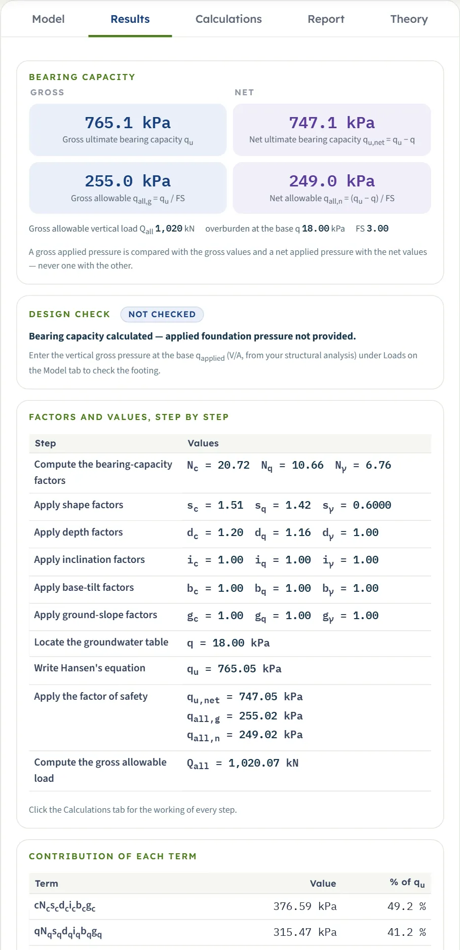
| Card | The example |
|---|---|
| Gross ultimate bearing capacity qu | 765.1 kPa |
| Net ultimate bearing capacity qu,net = qu − q | 747.1 kPa |
| Gross allowable qall,g = qu / FS | 255.0 kPa |
| Net allowable qall,n = (qu − q) / FS | 249.0 kPa |
| Gross allowable vertical load Qall | 1,020 kN |
Below the cards the Design check says NOT CHECKED until you enter qapplied. Then a table lists the factors step by step (Nc Nq Nγ, the shape, depth, inclination, base-tilt and ground-slope factors, the groundwater table, qu, the allowable pressures and Qall), and a table gives the contribution of each term with its share of qu. For a strip Qall is per metre of length (kN/m, tf/m or kip/ft).
The check
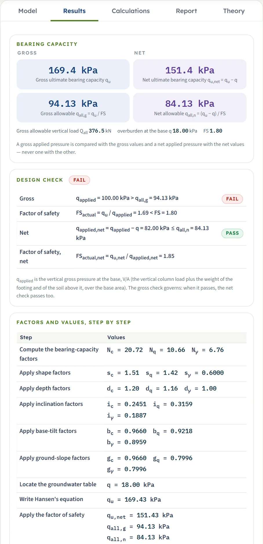
With qapplied entered the module compares gross with gross and net with net: the gross check qapplied ≤ qall,g and the actual factor of safety FSactual = qu / qapplied, and the net check qapplied − q ≤ qall,n . The gross line and the net line each carry a PASS or FAIL badge; the gross check governs: when it passes, the net check passes too. For the example, qapplied = 200 kPa passes with FSactual = 3.83 and 300 kPa fails with 2.55 (the gross allowable pressure is 255.0 kPa).
Using the numbers
- qu is the failure pressure, not a working value. Compare the applied pressure with the allowable pressure of the same kind: a gross applied pressure with qall,g , a net one with qall,n . The two are two conventions of applying the factor of safety.
- Pressures are in kPa, t/m² or ksf by the unit system; the same example gives 78.01 t/m² (SI · tf) and 15.98 ksf (US). The drawings stay in SI whatever the unit system.
- Changing the unit system after Analyze re-states the Results without a new run.
Warnings and notes
The bar carries a Warnings (n) button. For usual values the window reads “No warnings — the method’s assumptions hold for these inputs.” A caution, such as the sliding one below, opens the window by itself when you analyse and adds “— 1 warning” to the bar. A condition that stops the analysis is shown as a message, see Messages.
The Calculations tab, the report and the Theory tab
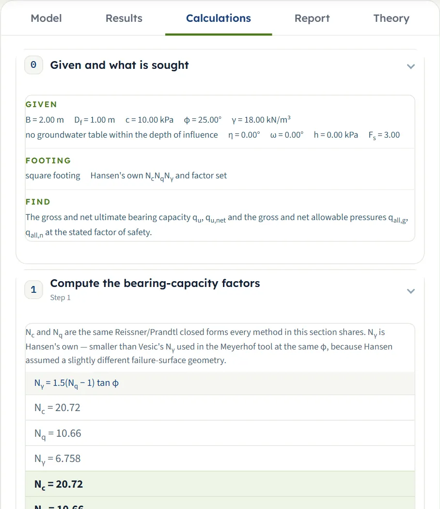
The Calculations tab opens with Given and what is sought and then writes out the working in numbered steps, each with the formulas and your numbers:
- Compute the bearing-capacity factors — Nc, Nq and Hansen’s Nγ = 1.5(Nq − 1) tan φ.
- Apply shape factors — sc, sq, sγ with B/L (the φ = 0 form s′c = 0.2B/L for an undrained soil).
- Apply depth factors — dc = 1 + 0.4k, dq = 1 + 2 tan φ (1 − sin φ)² k and dγ = 1, with k = Df/B, or arctan(Df/B) when Df/B is above 1. Around Df/B = 1 the step writes out that the two forms meet with a step of a few per cent.
- Apply inclination factors — from h/(qapplied + c cot φ); all 1 when h = 0 (and i′c = 0 in the φ = 0 form).
- Apply base-tilt factors — bc = 1 − η/147°, bq = e−2η tan φ , bγ = e−2.7η tan φ .
- Apply ground-slope factors — gc = 1 − ω/147°, gq = gγ = (1 − 0.5 tan ω)⁵.
- Locate the groundwater table — q and the unit weight of the self-weight term.
- Write Hansen’s equation — the three terms and qu, with the contribution of each term.
- Apply the factor of safety, Compute the gross allowable load, and, with qapplied, Check the applied foundation pressure, ending with the Answer.
The report
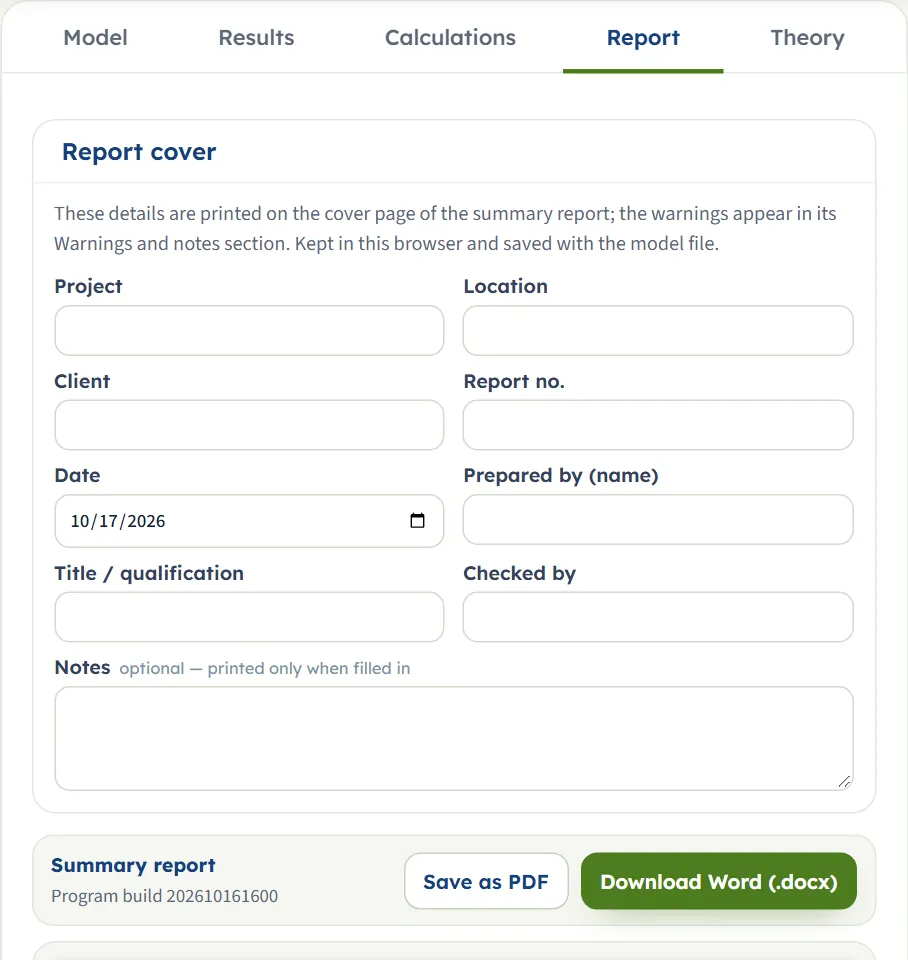
In the Report tab fill in the cover (project, location, client, report number, date, prepared by, title or qualification, checked by, and optional notes). The details are kept in this browser and saved with the model file. Save as PDF and Download Word (.docx) become available once the model is analysed; the preview below the buttons is the report itself.
The report has six parts: 1 Introduction and scope, 2 Input data (a table of the inputs with the section drawing), 3 Calculation (the steps of the Calculations tab), 4 Results (with the Capacity drawing), 5 Summary and 6 References; when the analysis carries a caution it has seven, with 5 Warnings and notes, 6 Summary and 7 References. It states the units used.
The Theory tab
The Theory tab explains Hansen’s equation in sections: why Hansen’s Nγ differs from the others (with a table against φ), the shape and depth factors, the inclination factors, the base-tilt and ground-slope factors, putting the equation together, the undrained case (φ = 0), how the module’s numbers were checked, and the reference.
Worked example: the module’s own example
The module opens on this example, so you can follow the numbers on your own screen.
| Section | Input | Value |
|---|---|---|
| Footing | Shape, B, Df | Square, B = 2 m, Df = 1 m |
| Soil | c, φ, γ | 10 kPa, 25°, 18 kN/m³ |
| Groundwater | Water table | None |
| Base tilt and ground slope | η, ω | 0°, 0° |
| Loads | h, qapplied | 0, empty |
| Analysis Settings | FS | 3 |
Step 1: the factors of the equation
Nq = eπ tan 25° tan²(45° + 25°/2) = 10.66, Nc = (Nq − 1)/tan 25° = 20.72 and Nγ = 1.5(Nq − 1) tan 25° = 6.758. For a square, B/L = 1: sc = 1 + Nq/Nc = 1.515, sq = 1 + sin 25° = 1.423, sγ = 1 − 0.4 = 0.600. With k = Df/B = 0.5: dc = 1 + 0.4 × 0.5 = 1.200, dq = 1 + 2 tan 25° (1 − sin 25°)² × 0.5 = 1.155, dγ = 1. The inclination, tilt and slope factors are 1.
Step 2: the three terms
qu = 376.6 + 315.5 + 73.0 = 765.1 kPa. The surcharge q = 18 × 1 = 18.0 kPa, so qu,net = 747.1 kPa. With FS = 3, qall,g = 765.1 / 3 = 255.0 kPa and qall,n = 747.1 / 3 = 249.0 kPa, and Qall = 255.0 × 2 × 2 = 1,020 kN. These are the cards of the Results tab.
An inclined case with a tilt and a slope
Change the example to η = 5°, ω = 5°, h = 50 kPa, qapplied = 100 kPa and FS = 1.8. With x = h/(qapplied + c cot φ) = 50 / (100 + 21.44) = 0.4117: iq = (1 − 0.5 × 0.4117)⁵ = 0.3159, ic = iq − (1 − iq)/(Nq − 1) = 0.2451 and, on the tilted base, iγ = (1 − (0.7 − 5/450) × 0.4117)⁵ = 0.1887. The base-tilt factors are bc = 1 − 5/147 = 0.9660, bq = e−2 × 0.08727 × tan 25° = 0.9218 and bγ = 0.8959; the ground-slope factors are gc = 0.9660 and gq = gγ = (1 − 0.5 tan 5°)⁵ = 0.7996. The terms are 86.1 + 73.4 + 9.9, so qu = 169.4 kPa and qall,g = 94.13 kPa. The module gives the same, and qapplied = 100 kPa is above 94.13 kPa: FAIL, FSactual = 1.69. The net check, 82.00 kPa against qall,n = 84.13 kPa, passes; the gross check governs.
Other unit systems
The same example reads 78.01 t/m² in SI · tf and 15.98 ksf in US: the same pressure in other units. Two checks entered in the units of the system, with the cohesion in the unit the box shows:
- US. A square footing of 6 ft at 3 ft depth, c = 300 psf, φ = 30° and γ = 120 pcf. Nc = 30.14, Nq = 18.40, Nγ = 15.07, sc = 1.610, sq = 1.5, sγ = 0.6, dc = 1.2, dq = 1.144; q = 0.36 ksf. The terms are 0.3 × 30.14 × 1.610 × 1.2 = 17.47, 0.36 × 18.40 × 1.5 × 1.144 = 11.37 and ½ × 0.12 × 6 × 15.07 × 0.6 = 3.26 ksf, so qu = 32.10 ksf. The module gives 32.10 ksf, qall,g = 10.70 ksf and Qall = 385.2 kip.
- SI · tf. A rectangle 1.5 × 3 m at 1 m depth, c = 0.1 kg/cm² (1 t/m²), φ = 30° and γ = 1.8 t/m³. B/L = 0.5: sc = 1.305, sq = 1.25, sγ = 0.8, dc = 1.267, dq = 1.192. The terms are 49.84 + 49.37 + 16.27 t/m², so qu = 115.5 t/m². The module gives 115.5 t/m², qall,g = 38.49 t/m² and Qall = 173.2 tf.
How each input changes the answer
Each row changes one thing in the example (a 2 m square footing at 1 m depth, c = 10 kPa, φ = 25°, γ = 18 kN/m³, no water, level, vertical load, FS = 3) and runs the module again. The numbers are the ones the module gives, so you can reproduce any row; pressures are in kPa.
| Change | qu | qall,g |
|---|---|---|
| The example: square 2 m, Df = 1 m, c = 10, φ = 25°, γ = 18, FS = 3 The reference | 765.1 | 255.0 |
| Shape: strip No shape correction: the cohesion and surcharge terms drop, the self-weight term rises | 592.0 | 197.3 |
| Shape: rectangle, L = 4 m Between the strip and the square | 678.5 | 226.2 |
| Df = 0 No surcharge term, and dc = 1 | 386.8 | 128.9 |
| Df = 2 m The surcharge term grows with the depth | 1228.2 | 409.4 |
| Df = 3 m Df/B above 1: the depth factors take the arctan form | 1579.5 | 526.5 |
| B = 3 m A wider footing: almost the same qu, because the depth factors fall as B grows | 766.5 | 255.5 |
| c = 0 The cohesion term vanishes | 388.5 | 129.5 |
| c = 20 kPa The cohesion term doubles | 1141.6 | 380.5 |
| φ = 0 (c = 10) Undrained form: Nc = 5.14, Nγ = 0 | 90.0 | 30.0 |
| φ = 30° Nc = 30.14, Nq = 18.40, Nγ = 15.07 | 1313.8 | 437.9 |
| φ = 35° The capacity more than triples | 2382.6 | 794.2 |
| γ = 20 kN/m³ Larger q and self-weight | 808.2 | 269.4 |
| Water table at Dw = 0.5 m, γsat = 19 Above the base: q and the self-weight term fall | 652.1 | 217.4 |
| Water table at the base, Dw = 1 m Only the self-weight term falls | 729.3 | 243.1 |
| Base tilt η = 10° bc, bq and bγ below 1 | 677.6 | 225.9 |
| Ground slope ω = 10° gc and gq = gγ below 1 | 595.8 | 198.6 |
| Ground slope ω = 20° A steeper slope, a lower capacity | 467.6 | 155.9 |
| η = 10° and ω = 10° Both reductions together | 533.0 | 177.7 |
| h = 20 kPa with qapplied = 100 kPa The inclination factors reduce all three terms | 476.3 | 158.8 |
| FS = 2 qu is the same; qall,g rises | 765.1 | 382.5 |
The pattern follows the equation. The friction angle moves the answer most among the rows (35° gives about three times the value at 25°); the depth, through q and the depth factors, comes next, and the cohesion term is proportional to c. A tilt of 10° takes 11 per cent off, a slope of 10° 22 per cent, and both together 30 per cent. The factor of safety does not change qu. A footing that is wider at a fixed depth is not always stronger, because k = Df/B falls: compare neighbouring widths before settling on one.
Messages: when the module stops, and what it cautions
The module checks the numbers before it calculates. When one cannot be used it stops, and nothing is calculated; the limits are shown in the units of the unit system chosen.
Input limits
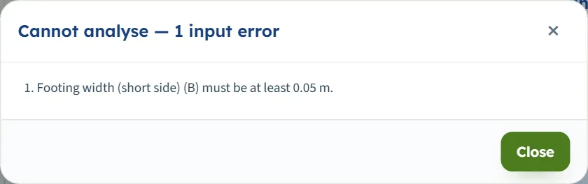
If an input is outside its limits or empty, pressing Analyze opens a window titled Cannot analyse — 1 input error (or 2 input errors …) that lists each message.
| When | Message |
|---|---|
| The width is below 0.05 m | “Footing width (short side) (B) must be at least 0.05 m.” |
| A value is empty | “Footing width (short side) (B) is missing.” |
| The friction angle is above 50° | “Friction angle (φ) must be at most 50°.” |
| The tilt is above 45° (the slope likewise) | “Base tilt from horizontal (η) must be at most 45°.” |
| The factor of safety is below 1 | “Factor of safety (FS) must be at least 1.” |
Conditions the equation cannot take
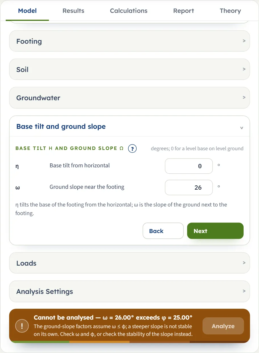
These stop the analysis with a bar that reads Cannot be analysed — … and a line saying what to do; the Analyze button is dimmed until you change the inputs.
| When | Message and what to do |
|---|---|
| A rectangle has L shorter than B | “Cannot be analysed — L = 1.00 m is shorter than B = 2.00 m”. Hansen’s shape factors take B as the shorter side: swap the two values. |
| ω is above φ (φ above 0) | “Cannot be analysed — ω = 26.00° exceeds φ = 25.00°”. The ground-slope factors assume ω ≤ φ; check the two angles, or check the stability of the slope instead. |
| h is above 0 and qapplied is empty | “Cannot be analysed — enter qapplied for this load case”. Enter qapplied or set h to 0. |
| h reaches qapplied + c cot φ | “Cannot be analysed — h = 130.00 kPa reaches v + c·cot φ = 121.45 kPa” (for qapplied = 100 kPa and the example soil). The inclination factors vanish there; reduce h, check qapplied, and check the footing against sliding. |
| φ = 0 and h reaches c | “Cannot be analysed — h = 15.00 kPa reaches the undrained base resistance c = 10.00 kPa” (for c = 10 kPa). Beyond h = c the base slides before it can fail in bearing: reduce h or check c, and check the footing against sliding. With c = 0 any h above 0 stops at φ = 0; at φ = 0 this stop replaces the sliding caution. |
| At φ = 0 the horizontal load, the tilt and the slope together outweigh the rest | “Cannot be analysed — 1 + s′c + d′c − i′c − b′c − g′c = -0.0332 ≤ 0” (a strip at the surface with c = 40 kPa, h = 39 kPa, qapplied = 100 kPa and η = ω = 45°). Reduce h, the tilt or the slope. |
| Water with γsat not above the unit weight of water | “Cannot be analysed — γsat ≤ γw — the submerged unit weight would not be positive”. Check γsat. |
The sliding caution
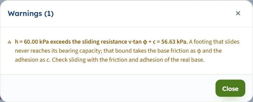
When h is above the sliding resistance qapplied tan φ + c the analysis still runs, and a caution opens by itself. With h = 60 kPa and qapplied = 100 kPa the window reads “h = 60.00 kPa exceeds the sliding resistance v·tan φ + c = 56.63 kPa.” and the bar reads “Analysed — FAIL … — 1 warning”. The bound takes the base friction as φ and the adhesion as c; check sliding with the friction and adhesion of the real base.
Good practice and common mistakes
- Give h and qapplied from the same load combination, with service (unfactored) loads: the inclination factors use their ratio, and the check uses the same qapplied.
- Put the footing weight and the soil on it into qapplied. It is the gross pressure at the base: the column load plus the weight of the footing and of the soil above it, over the base area.
- Compare like with like. Gross applied pressure against qall,g , net against qall,n ; the gross check is the stricter.
- Check sliding and the stability of the slope separately. The factors only reduce the capacity; the module cautions when h passes qapplied tan φ + c, and a footing on or near a slope needs a check of the slope as a whole.
- Use φ = 0 with the undrained cohesion for a clay under short-term loading; use drained parameters for the long term.
- Keep to one method’s numbers. Hansen’s Nγ is smaller than Vesic’s at the same φ (6.76 against 10.88 at 25°); do not mix factors of different methods.
- Watch Df/B near 1. The depth factors change form there, and the Calculations tab says so.
- Check the units after switching the system: type values in the units shown beside the boxes (cohesion in psf in the US system and in kg/cm² in SI · tf).
- Keep a record. The report is the record of an analysis; use Quick Save… or Save to file… to keep the model.
Frequently asked questions
What is Hansen’s equation for?
It gives the bearing capacity of a shallow footing and, besides the usual shape and depth corrections, corrects for an inclined load, a tilted base and ground that slopes away from the footing. The module writes every factor out and gives the gross and the net capacity.
How is it different from the Meyerhof module?
Hansen uses its own Nγ, which is smaller than Vesic’s at the same φ (6.76 against 10.88 at 25°), and its own inclination factors, which use the horizontal and the vertical pressure of one load case rather than an angle. Hansen’s module also takes a base tilt and a ground slope, which the Meyerhof module does not.
Why does it ask for the vertical pressure when I enter a horizontal load?
The inclination factors depend on h/(qapplied + c cot φ), the horizontal pressure against the vertical one of the same load case. Without qapplied the module stops with “enter qapplied for this load case”.
What is the difference between gross and net?
The gross pressures are the total pressure at the base. The net ones are what the footing adds to the overburden q that already acts at that level: qu,net = qu − q. The gross allowable pressure divides the whole capacity by FS, the net one only the part above q. Compare a gross applied pressure with the gross value and a net one with the net value.
What do the tilt and the slope do?
Both reduce the capacity. For the example, a tilt of 10° takes the qu from 765.1 to 677.6 kPa, a slope of 10° to 595.8 kPa, and both together to 533.0 kPa. They are limited to 45°, and the slope may not exceed φ.
Why does the module stop when the slope is steeper than φ?
The ground-slope factors assume ω ≤ φ, and a steeper slope is not stable on its own. The module says so and suggests checking the stability of the slope instead.
What happens at φ = 0?
The cohesion term takes Hansen’s additive form, Nc = 5.14, Nγ = 0 and the self-weight term is zero. For the example soil with φ = 0 the module gives qu = 90.0 kPa; a strip with c = 40 kPa gives 264.7 kPa.
How does the water table enter?
Through the surcharge q and the self-weight term. A table above the base lowers both, one at the base lowers the self-weight term, and one more than a width below the base has no effect.
Does a circular footing have its own factors?
It takes the shape factors of a square of the same B, where B is the diameter, so the example gives the same qu for the two. The plan area used for Qall is πB²/4.
Which units does it use?
SI · kN, SI · tf or US, switchable in the header at any time. Pressures are in kPa, t/m² or ksf, loads in kN, tf or kip (per metre or foot of length for a strip) and lengths in m or ft. Cohesion is in kPa, kg/cm² or psf. The drawings stay in SI.
What does the report contain?
A cover with your project details and the answer, then the parts introduction and scope, input data with the section drawing, the calculation step by step and results with the Capacity drawing, then, when the analysis carries a caution, a Warnings and notes part, and finally the Summary and References. It is saved as a PDF or a Word file once the model is analysed.
Does the module remember my inputs?
Yes. Every change is kept in the browser, and the page opens again on the model you last worked on, analysed and locked if you left it so. Reset to defaults brings back the example; Save to file and Quick Save keep copies.