

What the module calculates
Vesic gives the ultimate and the allowable bearing capacity of a shallow footing on one soil, by Vesic’s equation (1973, 1975). It draws the failure mechanism to scale under the footing, works out the bearing capacity factors and the corrections for the shape and the depth of the footing, the inclination of the load, the tilt of the base and the slope of the ground, and gives the gross and the net ultimate capacity and the gross and the net allowable pressure. You enter the pressure that the footing applies and the module checks it: PASS or FAIL.
The three terms are the cohesion term, the surcharge term (the soil above the base, q) and the self-weight term. What sets this module apart is the inclination factors: their exponent m is worked out from the B/L ratio of the footing and from the direction in which the horizontal load acts, and the base tilt and the ground slope have their own factors.
What you can describe
- A strip, square, rectangular or circular footing: the width B (the shorter side, or the diameter of a circle), for a rectangle the length L, and the founding depth Df.
- One soil below the footing with the cohesion c, the friction angle φ and the unit weight γ, and, if there is groundwater, the saturated unit weight γsat and the depth Dw of the water table.
- A tilted base (the angle η) and sloping ground next to the footing (the angle ω).
- One load case: the horizontal pressure h = H/A and the vertical gross pressure qapplied = V/A at the base, and the direction of the horizontal load, parallel to B or to L.
- The factor of safety FS.
Which bearing capacity module for which job
- A vertical load on level ground, with general or local shear: Terzaghi.
- Shape, depth and an inclined load, with Meyerhof’s inclination factors: Meyerhof.
- Hansen’s own factors (including his Nγ and shape factors) for the inclination, a footing near a slope or a tilted base: Hansen.
- This module when the exponent of the inclination factors should follow the footing’s own B/L and the direction of the load, with Vesic’s base-tilt and ground-slope factors.
- A strip footing in an earthquake: Seismic bearing capacity.
- The family page lists all five.
The module gives the bearing pressure. The settlement of the footing, its sliding along the base, the eccentricity of the load and the overall stability of a slope are checked with the matching modules and your own design checks; the Stresses in a soil mass family gives the stresses below a footing for settlement work.
Before you start: what you need
Have these ready from your design:
| What | Notes |
|---|---|
| The footing From: your foundation design | The shape, the width B (and the length L of a rectangle) and the founding depth Df. |
| The soil From: your soil investigation | c, φ and γ of the soil below the footing, in the terms of the analysis you follow (effective stress parameters for drained conditions, φ = 0 and the undrained c for a short-term clay). |
| The groundwater From: the borehole logs | The depth Dw of the water table below the ground surface and the saturated unit weight γsat; or none. |
| The tilt and the slope From: the drawings | η and ω in degrees; both 0 for a level base on level ground. |
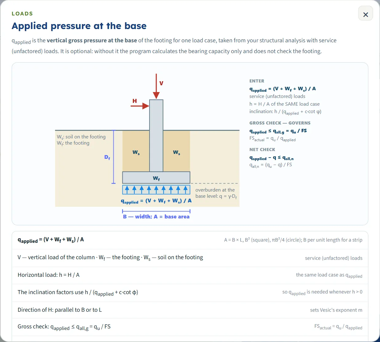
| The load From: your structural analysis | The horizontal pressure h = H/A and the vertical gross pressure qapplied = V/A of one load case, with service (unfactored) loads. qapplied includes the weight of the footing and of the soil above it. |
| The factor of safety From: your design basis | At least 1; 3 is the default. |
Quick start in eight steps
- Open the module and choose the units
Open Vesic from the Bearing Capacity family. Pick SI · kN, SI · tf or US in the header; you can change it at any time.
- Describe the footing
In Footing choose Strip, Square, Rectangular or Circular and type B (and L for a rectangle) and Df.
- Enter the soil and the groundwater
In Soil type c, φ and γ. In Groundwater choose Present and type γsat and Dw, or None.
- Enter the tilt, the slope and the load
In Base tilt and ground slope type η and ω (0 if level). In Loads choose the direction of the horizontal load, then type h and qapplied.
- Set the factor of safety
In Analysis Settings type FS.
- Press Analyze
Press Analyze at the foot of the Model tab. The drawing changes to the Capacity view and the bar reads PASS or FAIL.
- Read the answer
The Results tab gives qu, qu,net , qall,g and qall,n , the design check and every factor.
- Take the working and the report
The Calculations tab writes out the steps with your numbers; the Report tab saves a PDF or a Word file.
The screen: section, capacity and factors
The layout is the one every GeoTerva module shares, described in the workspace guide. The drawing has three views, chosen with the buttons above it:
- Section is the cross section through the footing, drawn to scale: the footing, the ground surface, the water table, Df and B, and the failure mechanism of the method for your φ: an elastic wedge under the base (I), a radial shear zone (II) and a passive wedge (III). It follows the inputs as you type. After Analyze it also shows qu under the base and the surcharge q.
- Capacity is empty until you press Analyze (it says “Press Analyze”). Afterwards it shows the three terms of qu as one bar with their shares, the gross pressures (qu, qall,g and qapplied) and the net pressures (qu,net , qall,n and the net applied pressure) as bars with the verdict, and all the factors of the equation.
- Factors draws Nc, Nq and Nγ against φ on a logarithmic scale, with the values at your φ. It follows φ and does not wait for Analyze.
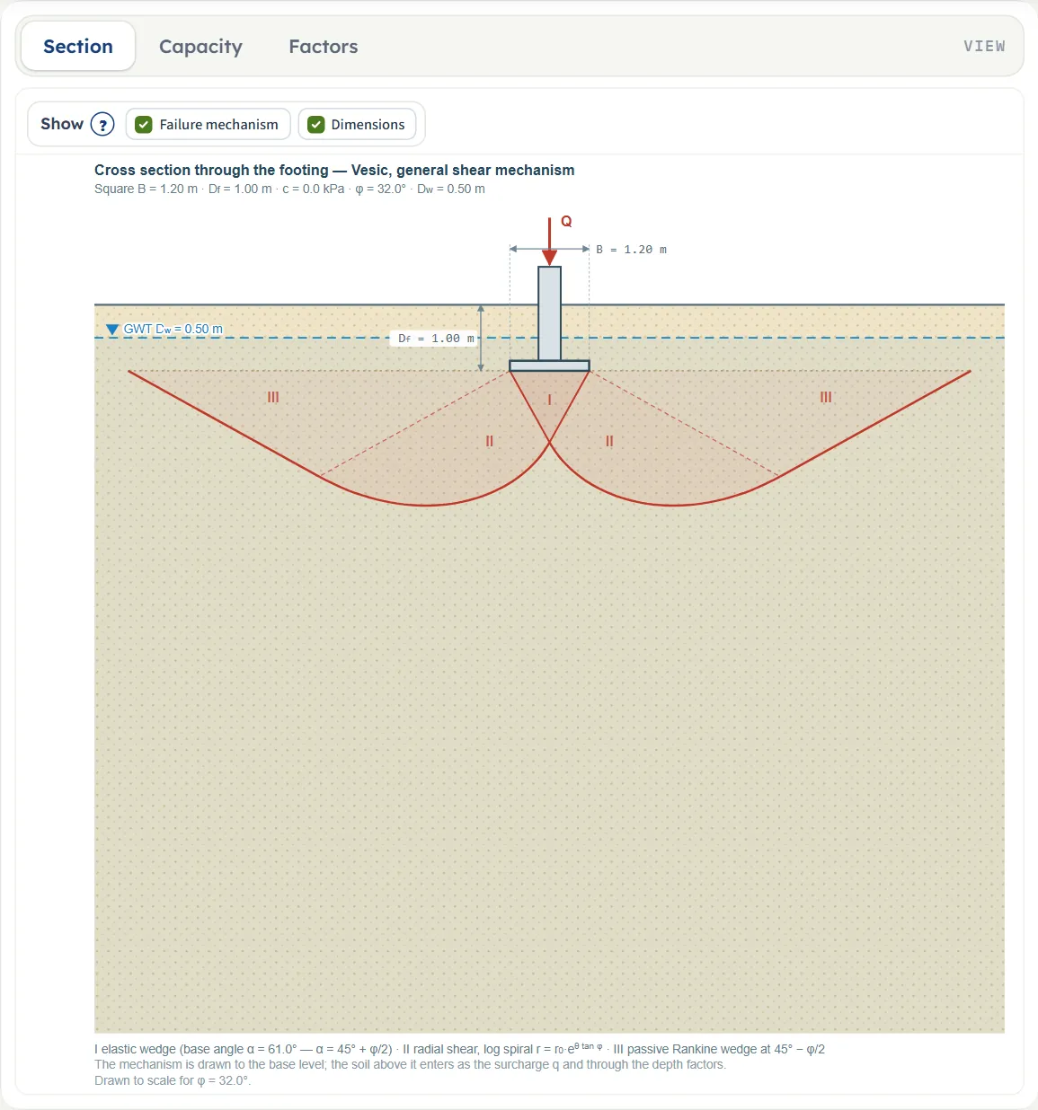
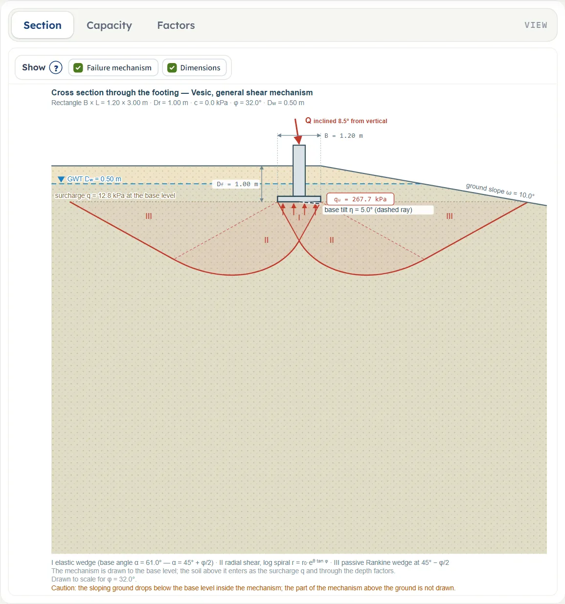
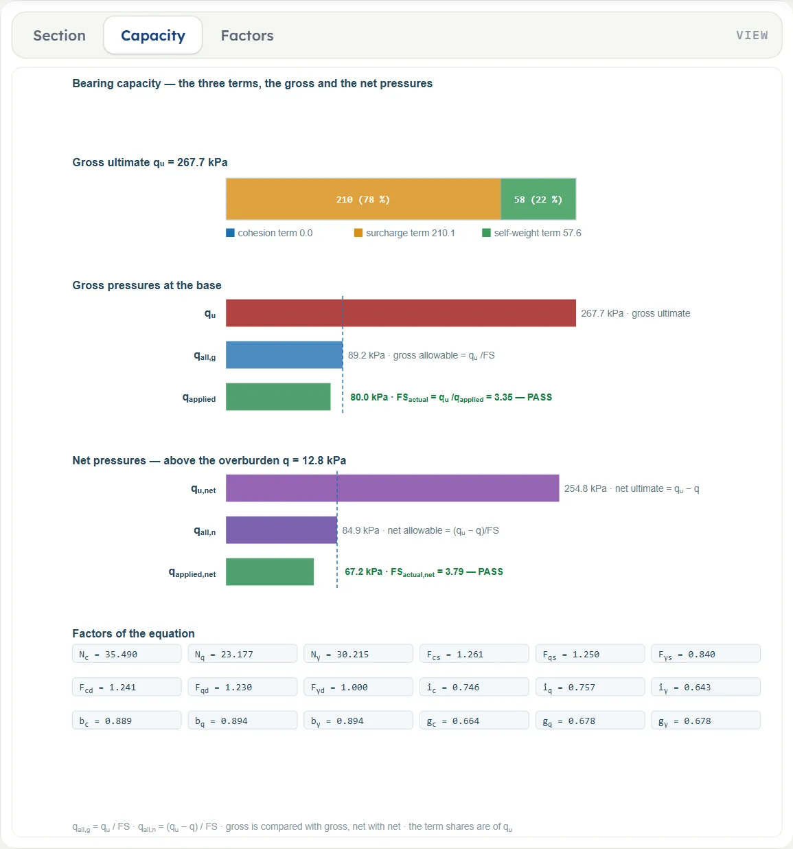
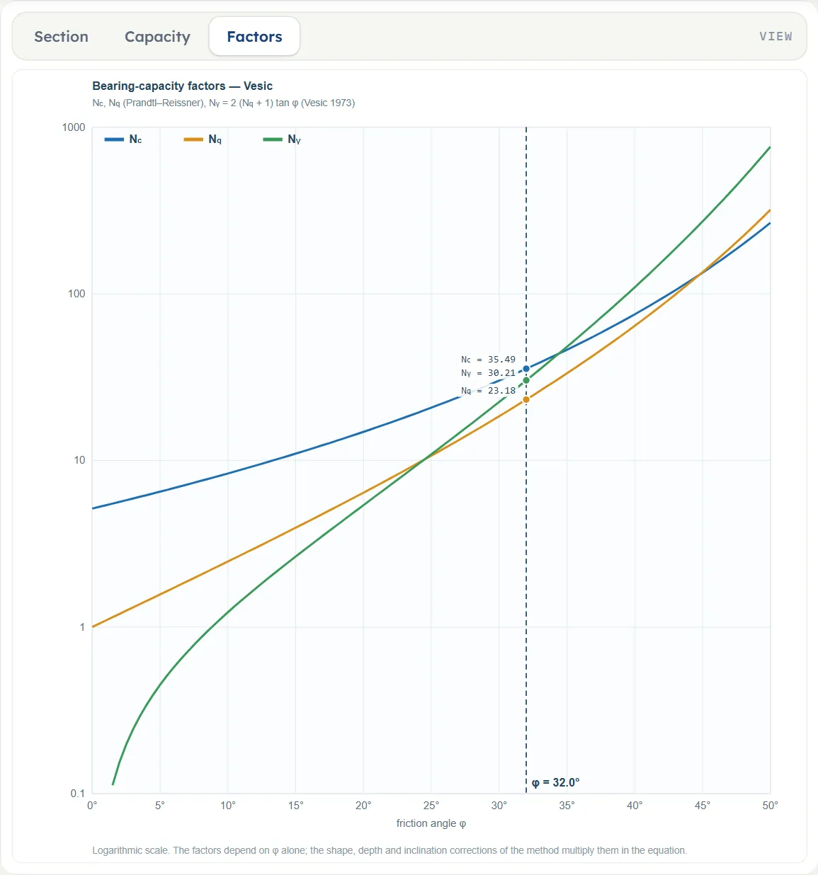
What the Section shows of the load, the tilt and the slope
- The load. A horizontal pressure with qapplied entered draws the load Q inclined from the vertical by the angle whose tangent is h/qapplied (8.5° for h = 12 and qapplied = 80 kPa). With Parallel to L and h above 0 the arrow stays vertical and is labelled “h acts along L (out of this section)”.
- The tilt. A base tilt η above 0 draws the base ray dashed and labels it “base tilt η = …°”.
- The slope. A ground slope ω above 0 draws the ground falling away from the footing and labels it “ground slope ω = …°”. When the slope drops below the base level inside the mechanism, a caution line under the drawing says that the part of the mechanism above the ground is not drawn.
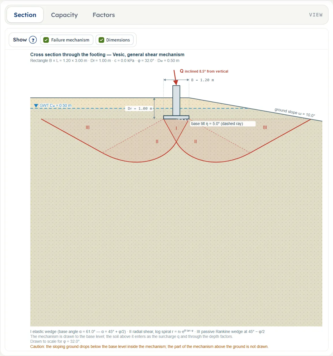
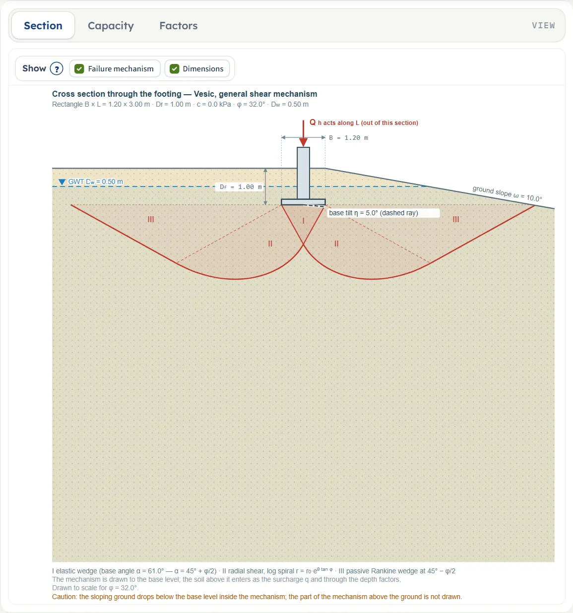
The Show chips
Above the Section a bar holds two chips, Failure mechanism and Dimensions, both on by default. Switching them off hides the zones and their legend, or the dimension lines of B, Df and the water table depth; the footing, the soil, the load and the value of qu stay. With the mechanism hidden the drawing says “The failure mechanism is hidden (Show: Failure mechanism).” The ? beside Show shows a tip saying that the drawing is to scale for your φ and is for display only. The Capacity and Factors views have no chips.

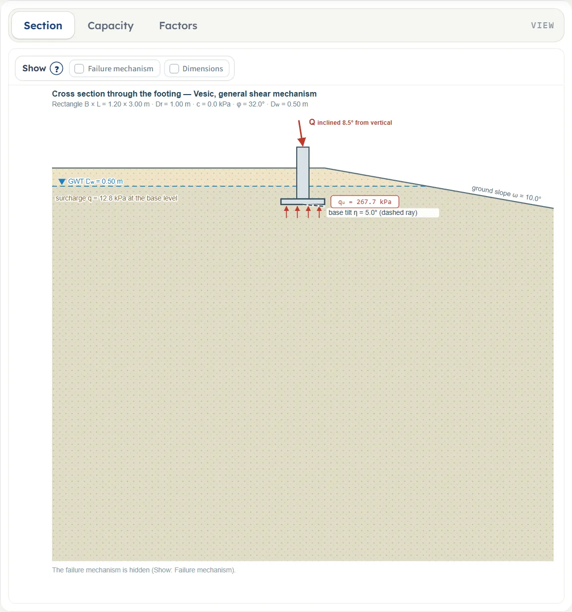
What you can drag
Nothing. The drawings are pictures of the model: the values are changed by typing them in the Model tab, and the drawing follows. There are no zoom buttons, and the mouse wheel does not zoom.
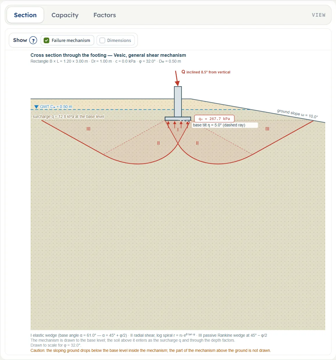
Entering the model, section by section
The Model tab has seven sections: Model data, Footing, Soil, Groundwater, Base tilt and ground slope, Loads and Analysis Settings. A section opens when you click its title; Next and Back walk you through them, and Analyze waits at the foot of the tab. In the tables a unit shown three times, such as kPa · t/m² · ksf, gives the units of SI · kN, SI · tf and US in turn. Defaults are shown in SI; in the other systems the boxes show the converted values. A box that is empty or outside its limit stops the analysis with a message, see Messages.
Model data
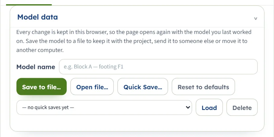
The first section holds the model name, Save to file…, Open file…, Quick Save… with its list and Load and Delete, and Reset to defaults. It works as described in the workspace guide. The note says that every change is kept in this browser, so the page opens again with the model you last worked on.
Footing
Choose the shape with four buttons. B is the width: the shorter side, or the diameter of a circle. L appears only when the shape is Rectangular, and must be at least B. A strip has no length: the module takes B/L = 0 for it, so it receives no shape correction, and its allowable load is given per metre of strip (kN/m, tf/m or kip/ft). A square and a circle take L = B, so B/L = 1.
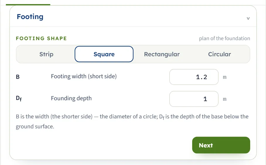
| Field | Unit | Default |
|---|---|---|
| Footing shape Strip, Square, Rectangular or Circular. | — | Square |
| Footing width (short side) B At least 0.05 m. | m · ft | 1.2 |
| Footing length (long side) L Shown for a rectangle only. At least 0.05 m, and not shorter than B. | m · ft | 1.2 |
| Founding depth Df The depth of the base below the ground surface. 0 or more. | m · ft | 1 |
Soil
One soil, below the footing, to the depth of the failure mechanism. The module takes the three values you type; it does not average layers.
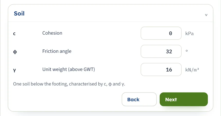
| Field | Unit | Default |
|---|---|---|
| Cohesion c 0 or more. | kPa · kg/cm² · psf | 0 |
| Friction angle φ From 0 to 50°. | ° | 32 |
| Unit weight (above GWT) γ At least 0.1 kN/m³. The moist unit weight of the soil above the water table. | kN/m³ · t/m³ · pcf | 16 |
Groundwater
Choose Present or None. With None the two boxes disappear and the moist γ is used for the surcharge and for the self-weight term. With Present, Dw is measured from the ground surface. Three read-outs follow the inputs: the surcharge q at the base, the water case (“above the base”, “within B below the base”, “deeper than B” or “none”) and Df / B. A water table below the base but within one width B of it gives the self-weight term a weighted unit weight; deeper than B below the base it has no effect.
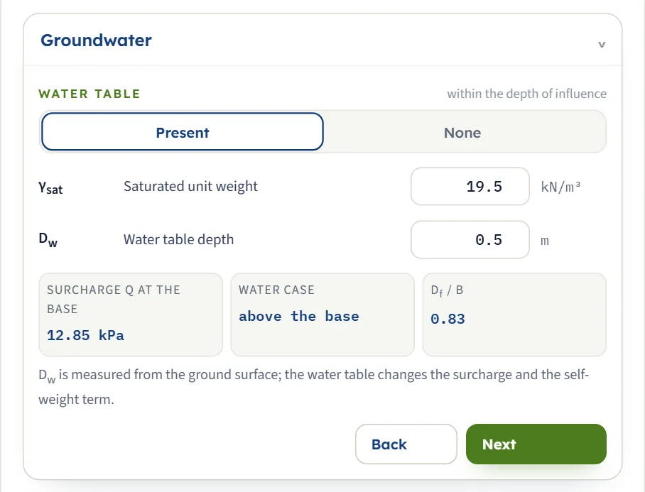
| Field | Unit | Default |
|---|---|---|
| Saturated unit weight γsat At least 0.1; it must exceed the unit weight of water (9.81 kN/m³). | kN/m³ · t/m³ · pcf | 19.5 |
| Water table depth Dw 0 or more, from the ground surface. | m · ft | 0.5 |
Base tilt and ground slope
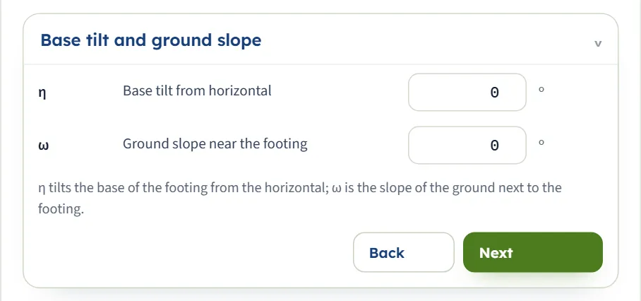
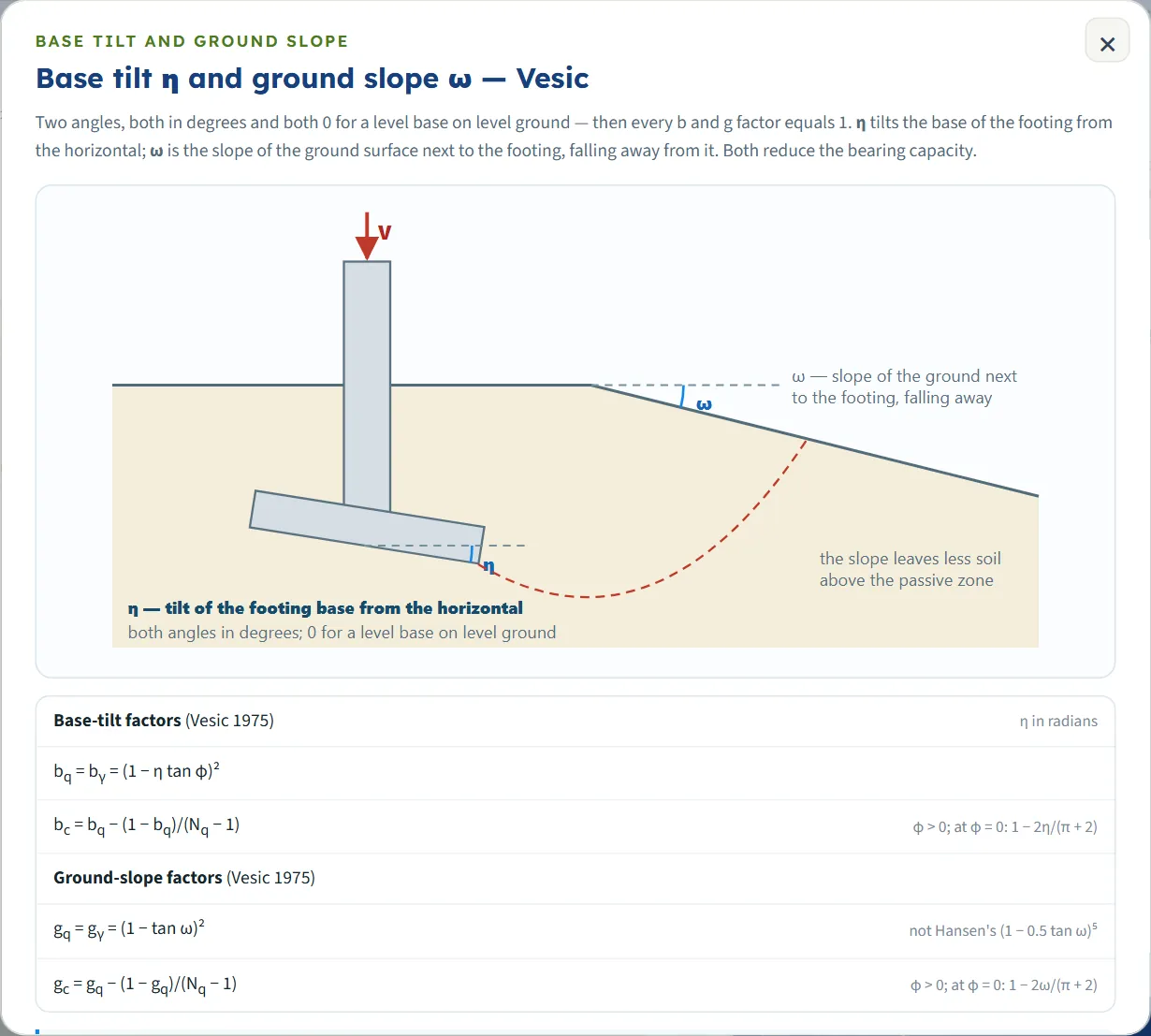
Two angles in degrees, both 0 for a level base on level ground; then every base-tilt and ground-slope factor equals 1. The ? beside the heading opens a window with a drawing of the two angles and the factors. η tilts the base of the footing from the horizontal; ω is the slope of the ground surface next to the footing, falling away from it. Both reduce the bearing capacity.
| Field | Unit | Default |
|---|---|---|
| Base tilt from horizontal η From 0 to 45°. | ° | 0 |
| Ground slope near the footing ω From 0 to 45°; with φ above 0 it may not exceed φ. | ° | 0 |
Loads
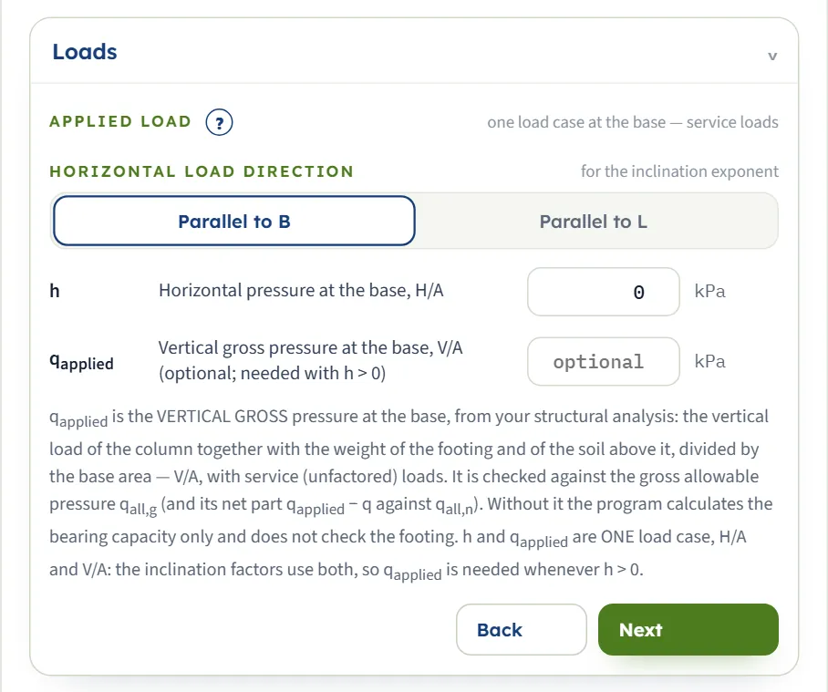
The load is one load case: the pressures h = H/A and qapplied = V/A of the same combination of service loads. The inclination factors use both, and the check of the footing uses qapplied. qapplied is the vertical gross pressure at the base: the vertical column load together with the weight of the footing and of the soil above it, divided by the base area. It is optional: without it the module gives the bearing capacity and does not check the footing; with h above 0 it is needed. Horizontal load direction has two buttons, Parallel to B and Parallel to L, and sets the exponent m. The ? beside Applied load opens a window with the drawing of the load case.
| Field | Unit | Default |
|---|---|---|
| Horizontal load direction Parallel to B or Parallel to L. | — | Parallel to B |
| Horizontal pressure at the base, H/A h 0 or more. | kPa · t/m² · ksf | 0 |
| Vertical gross pressure at the base, V/A qapplied Optional; 0 or more. Needed when h is above 0. | kPa · t/m² · ksf | empty |
Analysis Settings
One number: the factor of safety. The allowable pressures are the capacities divided by it.
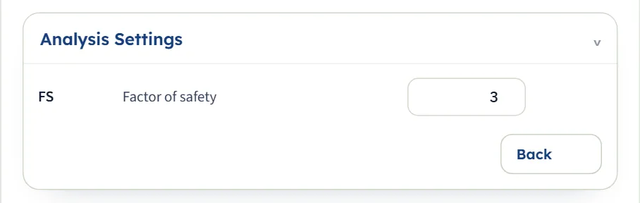
| Field | Unit | Default |
|---|---|---|
| Factor of safety FS At least 1. | — | 3 |
The inclination exponent, the tilt and the slope
Everything in the equation except the inclination, the tilt and the slope is the same as in the Meyerhof module: the factors Nc and Nq of Prandtl and Reissner, Nγ = 2 (Nq + 1) tan φ of Vesic, the shape factors of De Beer and the depth factors of Hansen. The Hansen module uses its own Nγ and shape factors, so the same footing gives a different answer there even with no inclination.
The exponent m: footing shape and direction of the load
The inclination factors raise the ratio x = h / (qapplied + c cot φ) to a power, and that power depends on the footing:
| B/L | Load ∥ B | Load ∥ L |
|---|---|---|
| 0 (strip) | 2.000 | 1.000 |
| 0.2 | 1.833 | 1.167 |
| 0.4 | 1.714 | 1.286 |
| 0.6 | 1.625 | 1.375 |
| 0.8 | 1.556 | 1.444 |
| 1 (square, circle) | 1.500 | 1.500 |
A strip is taken as B/L = 0: m = 2 for a load across the strip (B) and 1 for a load along it (L). A square and a circle have B/L = 1, so m = 1.5 whichever direction you choose, and the two direction buttons give the same qu. For a rectangle the direction matters: the same 1.2 m × 3 m footing with h = 20 and qapplied = 150 kPa gives qu = 458.2 kPa with the load parallel to B (m = 1.714) and 487.2 kPa parallel to L (m = 1.286). With h = 0 the inclination factors are 1 and the direction has no effect.
For φ = 0 the module uses ic = 1 − m h / (c Nc) and iq = iγ = 1.
Base tilt and ground slope
At φ = 0 the cohesion factors are bc = 1 − 2η/(π + 2) and gc = 1 − 2ω/(π + 2), the angles in radians, and the other two factors are 1 for the tilt, and (1 − tan ω)² for the slope. These are Vesic’s own forms; they differ from Hansen’s (for the ground slope, (1 − 0.5 tan ω)⁵), so the same footing gives a different answer in the two modules.
How the choices are made
- Direction of the load follows the way the structure pushes the footing. Choose the one that matches the horizontal load of the load case; for a square or circular footing it does not matter.
- h and qapplied come from one load combination. The module does not take the resultant Q/A: enter the pressure of its vertical component as qapplied.
- η and ω are 0 for a level base on level ground. The factors only reduce the capacity; a footing on or near a slope also needs the stability of the slope as a whole to be checked.
Analyze and read the results
Press Analyze. The bar counts through four steps (bearing capacity factors, corrections, groundwater, ultimate and allowable pressure), the inputs lock, and the drawing changes to the Capacity view. The page stays on the Model tab: open the Results tab for the answer. A message at the bottom of the window (“Analysed — PASS: see the Results tab and the Calculations.”) tells you the outcome for a moment.
- With qapplied entered, the bar reads Analysed — PASS: qapplied ≤ qall,g, FSactual = 3.35 (green) or FAIL: qapplied > qall,g, FSactual = … (red).
- Without qapplied it reads Analysed — bearing capacity calculated; applied pressure not provided, and nothing passes: the Design check shows NOT CHECKED.
- Edit inputs unlocks the inputs and clears the results; the unit system can be changed while the model is locked.

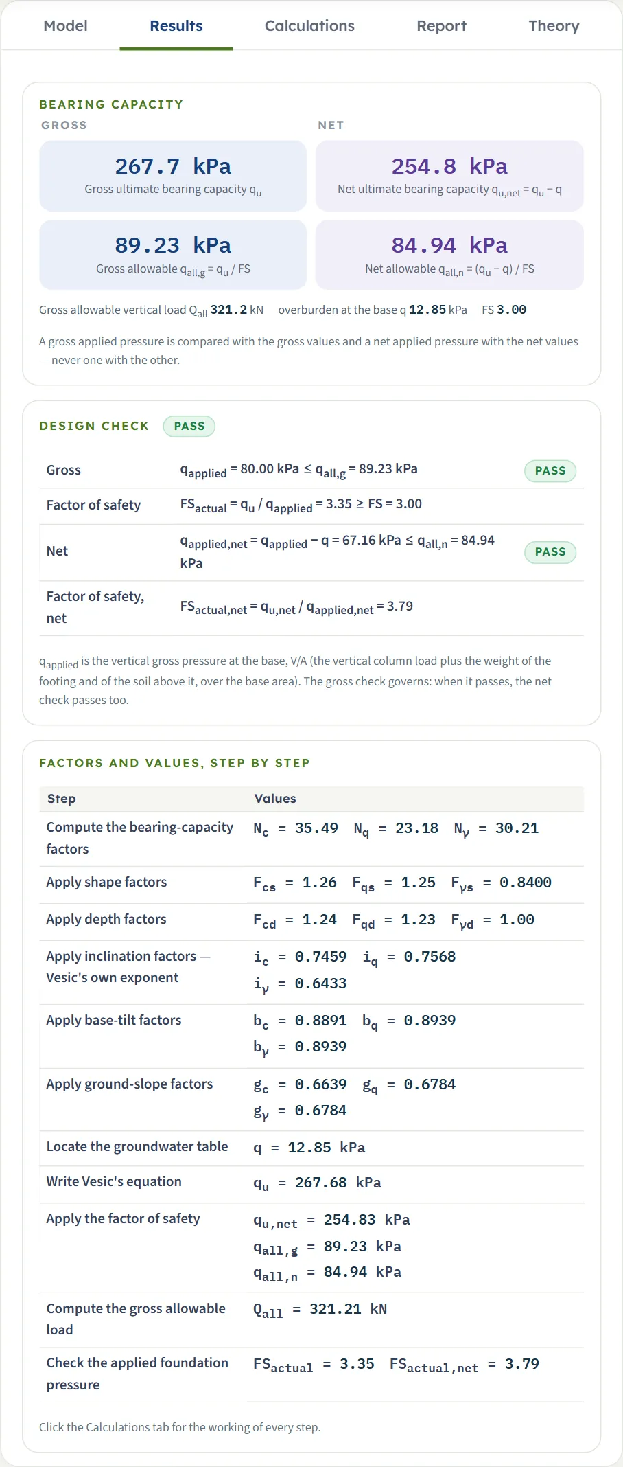
A line under the cards gives the gross allowable vertical load Qall (for a strip it is per unit length, in kN/m, tf/m or kip/ft), the overburden q at the base and FS.
| Card | Meaning | Example |
|---|---|---|
| Gross qu | Failure pressure | 700.5 kPa |
| Net qu,net | qu − q | 687.6 kPa |
| Gross qall,g | qu / FS | 233.5 kPa |
| Net qall,n | (qu − q) / FS | 229.2 kPa |
The Design check compares qapplied with qall,g and shows the actual factor of safety qu / qapplied; the same is done for the net pressures (qapplied − q against qall,n ). A gross pressure is compared with the gross values and a net one with the net values; the gross check governs. Below it Factors and values, step by step lists the factors of every step, and Contribution of each term gives the three terms of qu with their shares (in the default example 0.0 %, 85.0 % and 15.0 %).
Using the numbers
- qapplied is the pressure from service loads; the footing is checked against the allowable pressure, not against qu.
- The gross allowable load Qall is qall,g times the base area (B × L, πB²/4 for a circle, B per metre for a strip).
- Changing the unit system after Analyze re-states the numbers without a new run.
Warnings and notes
The bar carries a Warnings (0) button; with a caution it reads Warnings (1) and the window opens by itself when the analysis finishes. With nothing wrong it says “No warnings — the method’s assumptions hold for these inputs.” The conditions that stop the analysis and the cautions are listed under Messages.
The Calculations tab, the report and the Theory tab
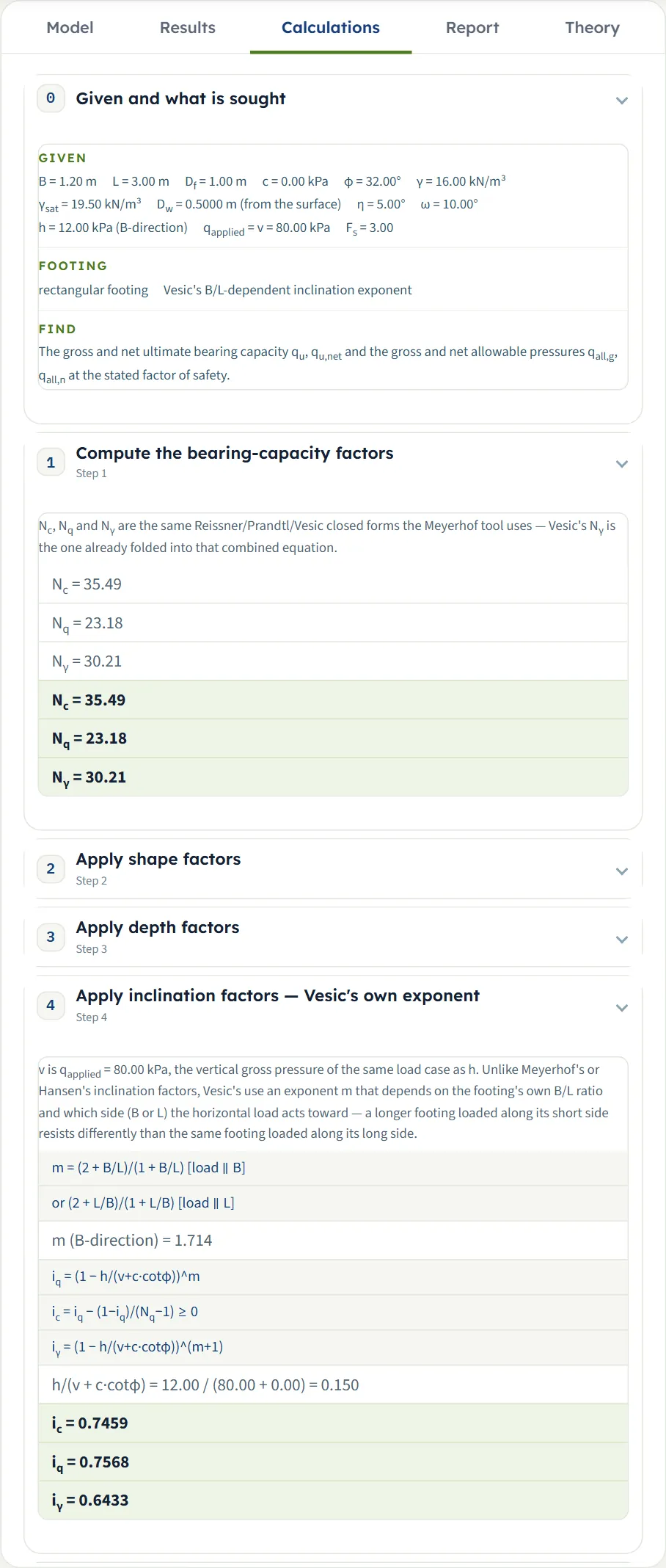
The Calculations tab opens with Given and what is sought and then writes out the working in eleven numbered steps; each opens and closes with its heading:
- Compute the bearing-capacity factors: Nc, Nq, Nγ.
- Apply shape factors: Fcs, Fqs, Fγs from B/L (all 1 for a strip).
- Apply depth factors: Fcd, Fqd, Fγd with k = Df/B, or its arctangent in radians when Df/B exceeds 1.
- Apply inclination factors: the exponent m, the ratio x and ic, iq, iγ; with h = 0 the step says that all three equal 1.
- Apply base-tilt factors: bc, bq, bγ.
- Apply ground-slope factors: gc, gq, gγ.
- Locate the groundwater table: the case, q and the unit weight of the self-weight term.
- Write Vesic’s equation: the three terms and qu, with a table of their shares.
- Apply the factor of safety: qu,net , qall,g , qall,n .
- Compute the gross allowable load: Qall.
- Check the applied foundation pressure: the gross and net checks and the actual factors of safety (only with qapplied).
The report
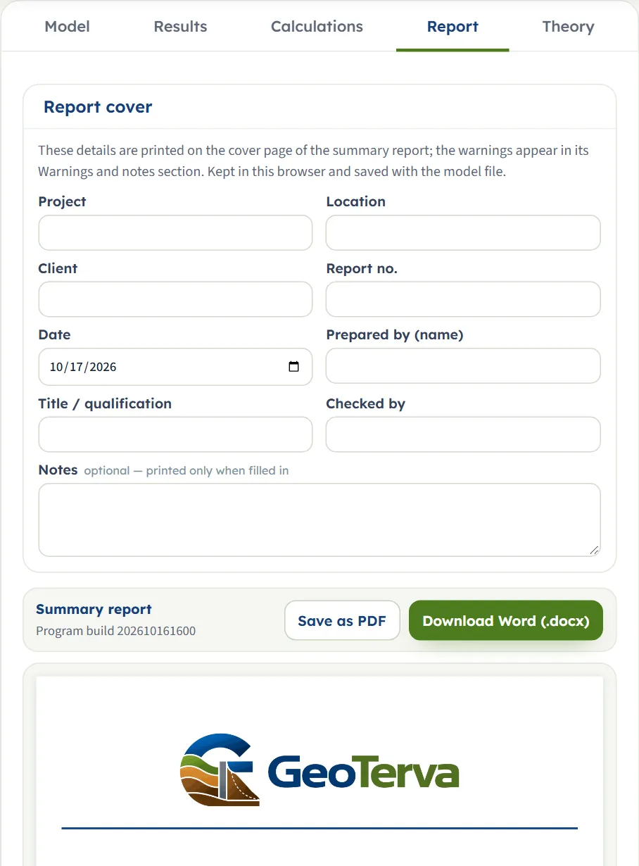
In the Report tab fill in the cover (project, location, client, report number, date, prepared by, title or qualification, checked by, and optional notes). Save as PDF and Download Word (.docx) produce the summary report; the preview below the buttons is the report itself. The details are kept in this browser and saved with the model file.
The report has six parts: 1 Introduction and scope, 2 Input data (a table of the inputs and the section drawing), 3 Calculation (the eleven steps), 4 Results (with the Capacity drawing), 5 Summary and 6 References; when the analysis carries a caution it has seven, with 5 Warnings and notes, 6 Summary and 7 References. It states the units used.
The Theory tab
The Theory tab explains the method in six sections: what Vesic contributed, the exponent that depends on the shape of the footing and the direction of the load (with a table of m against B/L), the base-tilt and ground-slope factors, what is unchanged from the other modules, how the numbers were checked, and the reference.
Worked example: the module’s own example, then an inclined load
The module opens on this example, so you can follow the numbers on your own screen.
| Section | Input | Value |
|---|---|---|
| Footing | Shape, B, Df | Square, 1.2 m, 1 m |
| Soil | c, φ, γ | 0 kPa, 32°, 16 kN/m³ |
| Groundwater | Present, γsat, Dw | 19.5 kN/m³, 0.5 m |
| Base tilt and ground slope | η, ω | 0°, 0° |
| Loads | h, qapplied | 0 kPa, empty |
| Analysis Settings | FS | 3 |
Step 1: the factors
With φ = 32°: Nq = eπ tan 32° tan²(45° + 16°) = 23.18, Nc = (Nq − 1) / tan 32° = 35.49, Nγ = 2 (Nq + 1) tan 32° = 30.21. For a square B/L = 1: Fcs = 1 + Nq/Nc = 1.653, Fqs = 1 + tan 32° = 1.625 and Fγs = 1 − 0.4 = 0.6. With k = Df/B = 0.8333: Fqd = 1 + 2 tan 32° (1 − sin 32°)² k = 1.230, Fcd = Fqd − (1 − Fqd) / (Nc tan 32°) = 1.241 and Fγd = 1. The inclination, tilt and slope factors are all 1.
Step 2: the groundwater
The water table (0.5 m) is above the base (1 m): q = 16 × 0.5 + (19.5 − 9.81) × 0.5 = 12.845 kPa, and the self-weight term takes the submerged unit weight γ′ = 19.5 − 9.81 = 9.69 kN/m³.
Step 3: the capacity
The module gives 700.5 kPa, with the shares 0.0 %, 85.0 % and 15.0 %. The net ultimate capacity is 700.46 − 12.845 = 687.6 kPa, and with FS = 3 the allowable pressures are 233.5 kPa (gross) and 229.2 kPa (net). The allowable load Qall = 233.49 × 1.2 × 1.2 = 336.2 kN.
The check
Enter qapplied = 200 kPa: the module reads PASS, FSactual = 700.46 / 200 = 3.50, and for the net pressures 187.16 kPa ≤ 229.20 kPa with 3.67. Enter 900 kPa: FAIL, FSactual = 0.7783.
An inclined load on a tilted base near a slope
Change the example to a rectangle L = 3 m, h = 12 kPa, qapplied = 80 kPa, η = 5°, ω = 10°, the direction parallel to B; the other inputs stay. Then B/L = 0.4 and m = (2 + 0.4) / (1 + 0.4) = 1.714; x = 12 / 80 = 0.15, iq = 0.851.714 = 0.7568, iγ = 0.852.714 = 0.6433, ic = 0.7568 − 0.2432 / 22.18 = 0.7459. The tilt gives bq = bγ = (1 − 0.08727 × tan 32°)² = 0.8939 and bc = 0.8891; the slope gives gq = gγ = (1 − tan 10°)² = 0.6784 and gc = 0.6639. With the shape factors of B/L = 0.4 (Fqs = 1.250, Fγs = 0.84) the terms are 210.11 and 57.57 kPa:
The module gives qu = 267.7 kPa, qall,g = 89.23 kPa, qall,n = 84.94 kPa, and the check reads PASS with FSactual = 267.68 / 80 = 3.35 (net 3.79); the allowable load is 89.23 × 1.2 × 3 = 321.2 kN. These are the figures on the pictures of this page. For comparison, a rectangle 1.2 m × 3 m with h = 20 and qapplied = 150 kPa on a level base and level ground gives 458.2 kPa (see the tables below).
Other unit systems
- US. B = 4 ft, L = 10 ft, Df = 3 ft, c = 100 psf, φ = 30°, γ = 110 pcf, γsat = 125 pcf, Dw = 5 ft, h = 0.4 ksf, qapplied = 3 ksf, FS = 3. A computation of Vesic’s equation with these values gives qu = 13.07 ksf; the module gives qu = 13.07 ksf, qall,g = 4.358 ksf, qall,n = 4.248 ksf and Qall = 174.3 kip.
- SI · tf. B = 1.5 m, L = 3 m, Df = 1.2 m, c = 0.5 kg/cm², φ = 30°, γ = 1.7 t/m³, γsat = 1.95 t/m³, Dw = 2 m, h = 2 t/m², qapplied = 15 t/m², FS = 3. The same computation gives 275.0 t/m²; the module gives qu = 275.0 t/m², qall,g = 91.68 t/m² and Qall = 412.6 tf.
- The default example in SI · tf gives qu = 71.43 t/m² and in US 14.63 ksf: the same 700.5 kPa in other units.
How each input changes the answer
Every row changes one thing in the example (a square footing, B = 1.2 m, Df = 1 m, c = 0, φ = 32°, γ = 16 and γsat = 19.5 kN/m³, water table at 0.5 m, FS = 3, no horizontal load) and runs the module again. The numbers are the ones the module gives, so you can reproduce any row. Pressures are in kPa.
| Change | qu | qall,g |
|---|---|---|
| The example The reference | 700.5 | 233.5 |
| Strip footing B/L = 0: no shape correction | 541.9 | 180.6 |
| Rectangle, L = 3 m B/L = 0.4 | 605.3 | 201.8 |
| Circular footing Same qu as the square; the load Qall differs by the area | 700.5 | 233.5 |
| φ = 28° | 420.2 | 140.1 |
| φ = 36° | 1,206 | 402.0 |
| c = 10 kPa The cohesion term appears | 1,428 | 476.1 |
| Df = 0 Footing on the surface: no surcharge | 134.0 | 44.67 |
| Df = 2 m | 1,196 | 398.5 |
| B = 2 m Wider: the self-weight term grows | 726.2 | 242.1 |
| γ = 18 kN/m³ | 746.8 | 248.9 |
| Groundwater None | 915.3 | 305.1 |
| Water table at 3 m More than B below the base: same as None | 915.3 | 305.1 |
| Water table at the surface (Dw = 0) | 554.3 | 184.8 |
| Factor of safety 2 qu stays; qall,g = qu / 2 | 700.5 | 350.2 |
The ground-water rows follow the water case: a table 0.5 m below the ground lowers qu from 915.3 to 700.5 kPa, and one at the surface to 554.3 kPa; a table deeper than B below the base acts as none.
| Change | qu | qall,g |
|---|---|---|
| The load, parallel to B m = 1.714 | 458.2 | 152.7 |
| Parallel to L m = 1.286 | 487.2 | 162.4 |
| h = 40 | 332.6 | 110.9 |
| h = 0 Vertical load only | 605.3 | 201.8 |
| η = 5° | 409.6 | 136.5 |
| ω = 10° | 310.9 | 103.6 |
| η = 5° and ω = 10° | 277.9 | 92.64 |
| Shape | qu | qall,g |
|---|---|---|
| Square m = 1.5 in either direction | 553.8 | 184.6 |
| Circular m = 1.5 | 553.8 | 184.6 |
| Strip, load across (B) m = 2 | 389.4 | 129.8 |
| Strip, load along (L) m = 1 | 449.3 | 149.8 |
| Change | qu | qall,g |
|---|---|---|
| η = 10° | 556.0 | 185.3 |
| η = 20° | 428.2 | 142.7 |
| ω = 10° | 475.2 | 158.4 |
| ω = 25° Close to the limit ω ≤ φ | 199.5 | 66.50 |
The pattern follows the equation. qu grows with φ and Df and falls when the water table rises into the failure zone. A horizontal load takes capacity away faster as h approaches qapplied + c cot φ, and by more for a strip loaded across it than for a square, because m is larger. A ground slope costs more than the same angle of base tilt: for φ = 32°, 10° of slope takes qu from 700.5 to 475.2 kPa and 10° of tilt to 556.0 kPa. For a clay with φ = 0 and c = 50 kPa (no water) the module gives qu = 425.3 kPa, and 299.1 kPa for a 1.2 × 3 m rectangle with η = 5°, ω = 10° and h = 20, qapplied = 100 kPa.
Messages: when the module stops, and what it notes
The module checks the numbers before it calculates. A condition it cannot calculate with is a stop; nothing is analysed, the bar reads Cannot be analysed and gives the reason and what to change, and Analyze stays unavailable until the inputs are changed.

| When | Message |
|---|---|
| L is shorter than B (rectangle) | “L = 0.8000 m is shorter than B = 1.20 m.” Swap the values, or enter the longer side as L. |
| h above 0 and qapplied empty | “enter qapplied for this load case.” Enter the gross vertical pressure, or set h = 0. |
| h reaches qapplied + c cot φ | “h = 160.00 kPa reaches v + c·cot φ = 100.00 kPa.” The inclination factors vanish there, and the base has slid long before it. Reduce h or check qapplied, and check the footing against sliding. |
| φ = 0 and h reaches c | “h = 60.00 kPa reaches the undrained base resistance c = 50.00 kPa.” (With c = 0 any h above 0 does.) Beyond h = c the base slides before it can fail in bearing. |
| φ is above 0 and ω is steeper than φ | “ω = 40.00° exceeds φ = 32.00°.” The ground-slope factors assume ω ≤ φ; check the stability of the slope instead. |
| γsat not above the unit weight of water | “γsat ≤ γw — the submerged unit weight would not be positive.” Check γsat. |
A value outside its limit or an empty box gives a window titled Cannot analyse — 1 input error (or more) when you press Analyze, listing each message in the units of the unit system:
| When | Message |
|---|---|
| η or ω above 45° | “Base tilt from horizontal (η) must be at most 45°.” (the same for the ground slope) |
| φ above 50° | “Friction angle (φ) must be at most 50°.” |
| FS below 1 | “Factor of safety (FS) must be at least 1.” |
| A box empty | “Footing width (short side) (B) is missing.” (the same for any required box; qapplied may stay empty) |
The caution
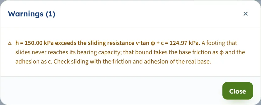
When φ is above 0 and h exceeds the sliding resistance qapplied tan φ + c but is still below qapplied + c cot φ, the module calculates and adds a caution: “h = 150.00 kPa exceeds the sliding resistance v·tan φ + c = 124.97 kPa. A footing that slides never reaches its bearing capacity; …” Check sliding with the friction and the adhesion of the real base. The Warnings window opens by itself after Analyze and the button reads Warnings (1). The check against qapplied is made as usual.
Notes in the working
- Df/B near 1. The depth factors use k = Df/B up to 1 and its arctangent above; the working notes that qu changes by a few per cent as Df/B crosses 1 (705.2 kPa at B = 1 m and Df = 1 m, 674.7 kPa at B = 0.9 m).
- ic below 0. The cohesion factor is held at 0.
Good practice and common mistakes
- Enter the pressure of the vertical component. qapplied is V/A with the weight of the footing and of the soil above it, from service loads. Do not enter the resultant.
- Keep h and qapplied in one load case. Combining the h of one combination with the qapplied of another gives inclination factors that belong to no load.
- Choose the direction for the rectangle. The exponent differs by about 0.4 between the two directions of a footing with B/L = 0.4; for a square it makes no difference.
- Gross against gross, net against net. The check does this for you; keep to one convention in your report.
- Check sliding and the slope. A base that slides never reaches its bearing capacity, and a footing near a slope needs the stability of the slope as a whole to be checked as well; the module gives the bearing pressure.
- Keep ω within φ and use the soil parameters of the analysis. Effective stress parameters for a drained case; φ = 0 with the undrained c for a short-term clay.
- Watch the water table. It lowers qu when it is above the base or within B below it; the read-outs in Groundwater show which case you are in.
- Compare methods. The same footing in Hansen and Meyerhof shows how much the method itself contributes.
- Keep a record. The report is the record of an analysis; Quick Save… or Save to file… keep the model.
Frequently asked questions
What does the module calculate?
The ultimate bearing capacity qu of a shallow footing on one soil by Vesic’s equation, the net capacity qu − q, and the gross and net allowable pressures at your factor of safety. With the applied pressure qapplied entered it gives PASS or FAIL. For the default example qu = 700.5 kPa and qall,g = 233.5 kPa.
What is the exponent m?
The power in the inclination factors: m = (2 + B/L) / (1 + B/L) for a horizontal load parallel to B and (2 + L/B) / (1 + L/B) for a load parallel to L. It is 2 or 1 for a strip, 1.5 for a square or a circle, and 1.714 or 1.286 for a footing with B/L = 0.4.
Which direction do I choose for the horizontal load?
The direction in which the horizontal load H acts relative to the footing: parallel to the width B or to the length L. It matters for a rectangle and a strip; for a square and a circle both give the same answer. With h = 0 it has no effect.
What do I enter as qapplied, and is it required?
The vertical gross pressure at the base, V/A, from service loads, including the weight of the footing and of the soil above it. It is optional: without it the module gives the capacity and nothing passes. With a horizontal pressure h above 0 it is required, because the inclination factors use h and qapplied together.
What do the base tilt and the ground slope do?
They reduce the capacity through the factors b and g: bq = bγ = (1 − η tan φ)² and gq = gγ = (1 − tan ω)². For the example, a slope of 10° gives qu = 475.2 kPa and a tilt of 10° gives 556.0 kPa, against 700.5 kPa on level ground.
Why does the module stop when ω is larger than φ?
The ground-slope factors assume ω ≤ φ; a steeper slope is not stable on its own. Check the stability of the slope instead. The tilt and the slope are accepted up to 45°.
What is the difference between gross and net?
The gross pressures include the overburden q at the base level; the net ones are what the footing adds to it. qu,net = qu − q and qall,n = (qu − q) / FS. A gross applied pressure is compared with the gross allowable pressure and a net one with the net; the gross check governs.
How does groundwater enter?
With the water table above the base the surcharge uses the submerged weight below it and the self-weight term takes the submerged unit weight. Below the base but within B the self-weight term takes a weighted unit weight; deeper than B it has no effect. For the example the water table at 0.5 m gives qu = 700.5 kPa against 915.3 kPa without water.
Can I drag the footing or zoom the drawing?
No. The drawings are pictures of the model; you change the model by typing in the Model tab, and the drawing follows. The Show chips switch the failure mechanism and the dimensions on and off.
Which units does it use?
SI · kN, SI · tf or US, switchable in the header at any time. Pressures are in kPa, t/m² or ksf, cohesion in kPa, kg/cm² or psf, unit weights in kN/m³, t/m³ or pcf, lengths in m or ft. The default example gives 700.5 kPa, 71.43 t/m² or 14.63 ksf.
Does the module remember my inputs?
Yes. The values you type are kept in the browser and the page opens again on the model you last worked on. A model that was analysed reopens analysed. Reset to defaults brings back the example; Save to file and Quick Save keep copies.
What does the report contain?
A cover with your project details and the answer, then six parts (seven when the analysis carries a caution, which adds warnings and notes): introduction and scope, input data with the section drawing, the calculation step by step, results, summary and references. It is saved as a PDF or a Word file.