

What the module calculates
Elastic settlement — granular gives the immediate settlement of a flexible foundation that rests on layers of sand and gravel. Granular layers are permeable: the water leaves as fast as the load is applied, so the soil settles drained, with the drained modulus E′ and Poisson’s ratio ν′, and there is no consolidation to add. The settlement is the integral of the vertical strain under the foundation:
The stresses are those of an elastic half-space (Boussinesq). The integral is evaluated in closed form with the influence factors of Steinbrenner (1934), layer by layer, so that every layer uses its own E′ and ν′. The settlement is summed from the foundation level down to the calculation depth zlim.
What you can describe
- A foundation that is a rectangle B × L or a strip of width B, flexible, carrying a uniform gross pressure qgross at the foundation level.
- A profile of granular layers from the ground surface down, each with its unit weights, E′ and ν′.
- The water table depth, and an excavation whose overburden is taken off the gross pressure.
- The calculation depth: the depth where the stress increase has fallen to a share p of q (the influence depth), or the bottom of the profile with a rigid base below it.
The module gives the settlement at the centre and at the corner (the edge of a strip) of the flexible foundation, the settlement of a rigid foundation (0.93 times the centre), the share of each layer and the settlement of every slice, draws the section and colour bands of stress, modulus, strain and settlement, writes out the working and prepares a PDF or Word report.
Which settlement module for which job
- Clay layers that settle undrained, with Eu and ν = 0.5: Elastic settlement, cohesive.
- The slow settlement of clay as it consolidates: Consolidation settlement.
- A profile that mixes clay and sand, with the immediate and the consolidation settlement together and the settlement–time curve: Settlement 2D.
- The stress increase itself at a point: Stress under a rectangular load.
- The bearing resistance of the same foundation: Bearing capacity.
Before you start: what you need
Have these ready from your investigation and your design:
| What | Notes |
|---|---|
| The profile | Layer depths from the ground surface, a name, the unit weight γ above the water table and γsat below it for each layer. Every layer is granular. |
| E′ and ν′ of each layer | The drained modulus and Poisson’s ratio, from tests or correlations. The help window Choosing E and ν gives ν′ commonly 0.25 – 0.35. Split a thick layer when its stiffness grows with depth. |
| The foundation | Width B, length L (or a strip), the gross pressure qgross at the foundation level. |
| The excavation and the water table | The excavation depth Dexc (the foundation level) and the depth zw of the water table below the ground surface. |
| The depth rule | The share p of q left at the calculation depth (10 % is common practice), or a rigid stratum at the bottom of the profile. |
Quick start in seven steps
- Open the module and choose the units
Open Elastic settlement — granular from the Settlement family. Pick SI · kN, SI · tf or US in the header, and the sign convention of the settlement beside it.
- Describe the soil profile
In Soil profile type the depth of the bottom of each layer, its name and its unit weights. In Elastic parameters type E′ and ν′ of the layers that will be compressed.
- Set the water table and the excavation
Type the water table depth in Groundwater and choose No or Yes in Excavation with its depth.
- Describe the foundation
In Foundation choose Rectangle / raft or Strip and type B, L and qgross. The net pressure qnet is shown under the boxes.
- Choose the calculation depth
In Analysis Settings choose Influence depth (Δσ = p · q) and p, or Bottom of the profile.
- Press Analyze
Press Analyze at the foot of the Model tab. The inputs lock, the drawing moves to the Settlement view and the bar reads Analysed.
- Read the answer
The Results tab gives the centre, corner and rigid settlement and the table by layer and by slice. Calculations shows the working of any slice; Report saves a PDF or a Word file.
The screen: three views of the section
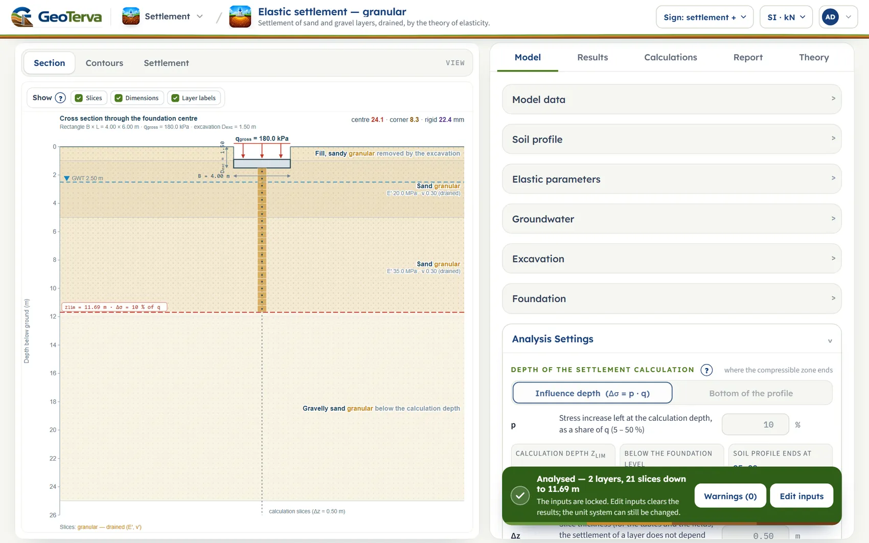
The layout is the one every GeoTerva module shares, described in the workspace guide. This module has three views of the section through the foundation centre, chosen with the buttons above the drawing. The drawing is a picture of the model: nothing can be dragged, and the drawing has no zoom or pan. You change the model in the Model tab and the drawing follows at once.
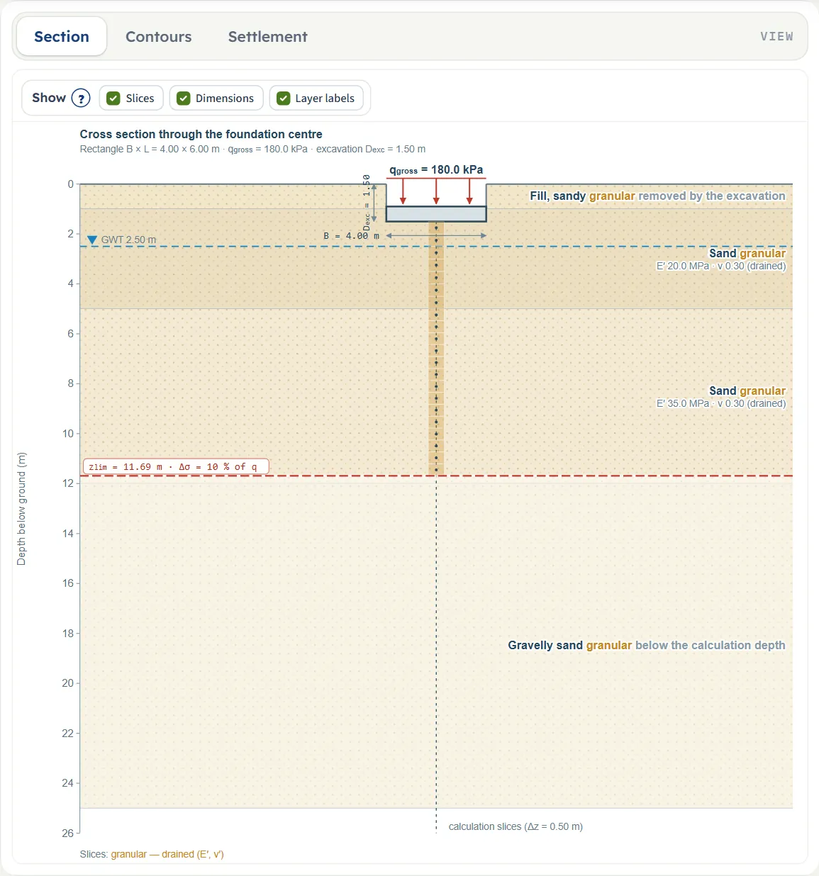
- Section shows the profile, the water table, the excavation, the foundation with its pressure, the calculation slices on the centre line and the calculation depth zlim (a dashed red line). It is available before and after Analyze.
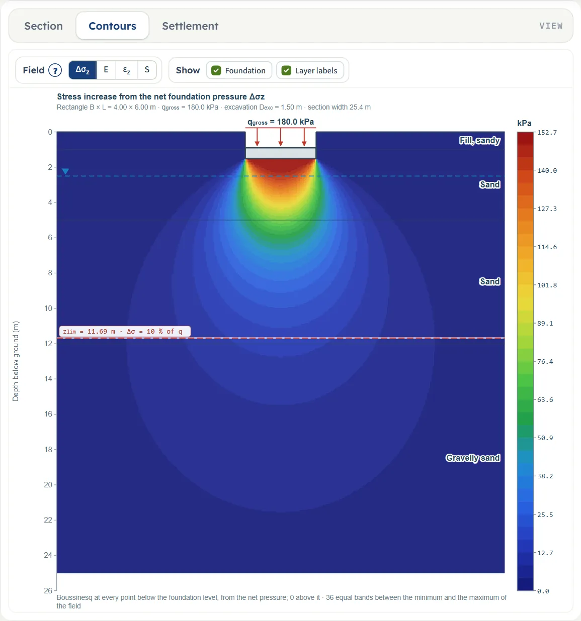
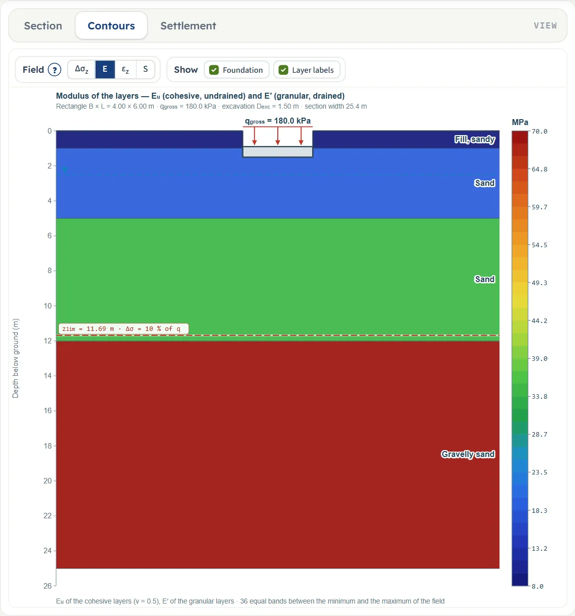
- Contours paints a field over the section, on the plane through the centre: the stress increase Δσz, the modulus E, the strain εz or the settlement S. Until you press Analyze it says “Press Analyze”.
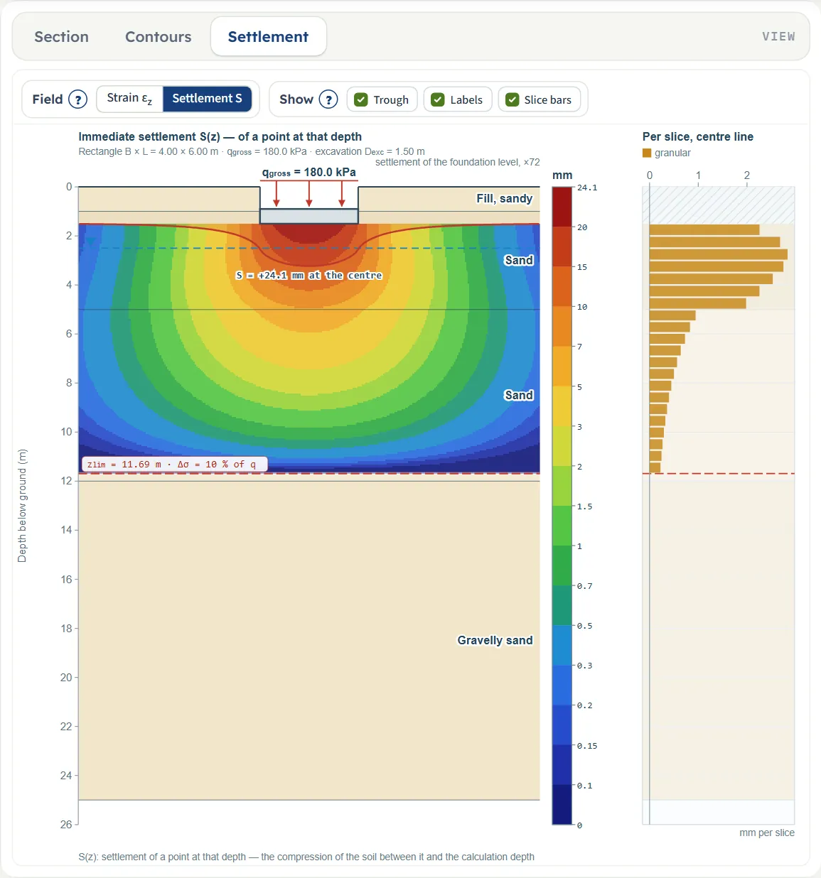
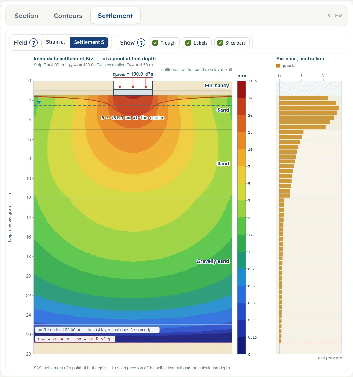
- Settlement shows the settlement S of a point at each depth (the compression of the soil between that point and the calculation depth) or the strain εz, the settlement trough of the foundation level and a bar for every slice on the centre line.
The Show and Field chips
| View | Chips |
|---|---|
| Section | Show: Slices, Dimensions, Layer labels |
| Contours | Field: Δσz, E, εz, S · Show: Foundation, Layer labels |
| Settlement | Field: Strain εz, Settlement S · Show: Trough, Labels, Slice bars |
The chips only change what is drawn. The (?) beside Show and Field explains each. Pointing at a slice on the Section view or a bar on the Settlement view shows its depth and, after Analyze, its settlement.

Colour bands
The stress increase and the modulus are painted in 36 equal bands between the smallest and the largest value of the field, with the legend beside the drawing. The strain and the settlement fall off quickly with depth, so they are painted in classes (1, 1.5, 2, 3, 5 and 7 times a power of ten, from 1/300 of the maximum upward): small values at depth keep colours of their own. The settlement field is zero below the calculation depth.
Entering the model, section by section
The Model tab has seven sections. They open one at a time as an accordion (click a title); Next and Back at the foot of a section walk you through them, and Analyze waits at the bottom of the tab. Model data is separate from the inputs. A value is taken when you leave the box or press Enter. The tables give the default of the example, in SI; units follow the unit system chosen in the header (the boxes convert).
Model data
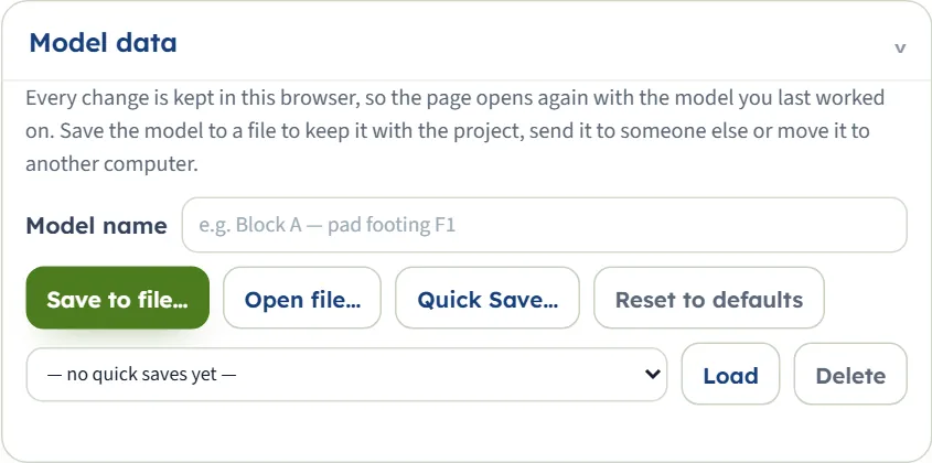
The model is kept in the browser after every change, so the page opens again on the model you last worked on, analysed or not, with a line such as “Opened with the model you last worked on (date and time), analysed. “Reset to defaults” starts again from the example project.” The unit system and the sign convention are remembered as well.
- Model name is a free name for the model.
- Save to file… writes the model to a .gtrv file; Open file… reads one. A file that is not a model gives “Not a model file: no model inputs found in the file”. A file with a layer of another kind opens with a note, for example “this module takes granular layers only: Clay was read as granular — check E′ and ν′”.
- Quick Save… asks for a name and keeps this version in the list beside Load and Delete; a name that exists asks before it is replaced. Load with nothing chosen says “Choose a saved model first.”
- Reset to defaults puts the example back and says “The inputs are back at the module defaults, and this is now the model kept in the browser.”
Soil profile
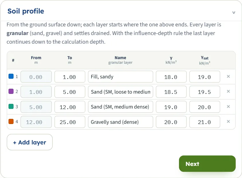
One row for each layer, from the ground surface down. From is read-only: it is the bottom of the layer above (0 for the first). You type To, the Name and the unit weights. A To that is not below the layer’s own From is ignored and the box returns to the old value. + Add layer appends a layer starting at the bottom of the last one, 2 m thick, named “Layer 5”, “Layer 6”…, with γ = 19.0 and γsat = 20.0 kN/m³. The × deletes a layer (the only remaining layer cannot be deleted); the layers below move up.
The four layers of the example are Fill, sandy (0–1 m), Sand loose to medium dense (1–5 m, γ 18.5, γsat 19.5), Sand medium dense (5–12 m, 19.0 and 20.0) and Gravelly sand dense (12–25 m, 20.0 and 21.0). A layer is granular by definition here, so there is no Type column.
| Field (unit) | First layer | Range |
|---|---|---|
| To m · ft | 1.00 | below From |
| γ kN/m³ · t/m³ · pcf | 18.0 | above zero |
| γsat kN/m³ · t/m³ · pcf | 19.0 | above zero |
Elastic parameters
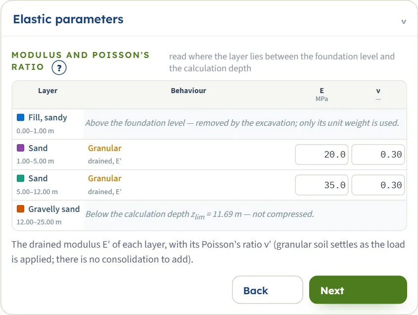
One row for each layer with the layer name and depths, the behaviour (granular, drained, E′) and two boxes. Only a layer that lies between the foundation level and the calculation depth has boxes; a layer above the foundation level says “Above the foundation level — removed by the excavation; only its unit weight is used.”, a layer below says “Below the calculation depth zlim = 11.69 m — not compressed.” These notes follow the model as you edit it. The (?) opens Choosing E and ν.
ν′ is limited to 0.49 when you type a larger value. E′ blank or zero stops the analysis (see Messages). The first layer of the example has E′ = 8 MPa and the fourth 70 MPa; they come into play when the foundation level or the calculation depth changes.
| Field (unit) | Example | Range |
|---|---|---|
| E′ MPa · kg/cm² · ksf | 20.0 and 35.0 (layers 2 and 3) | above zero |
| ν′ — | 0.3 | 0 to 0.49 |
Groundwater, Excavation and Foundation
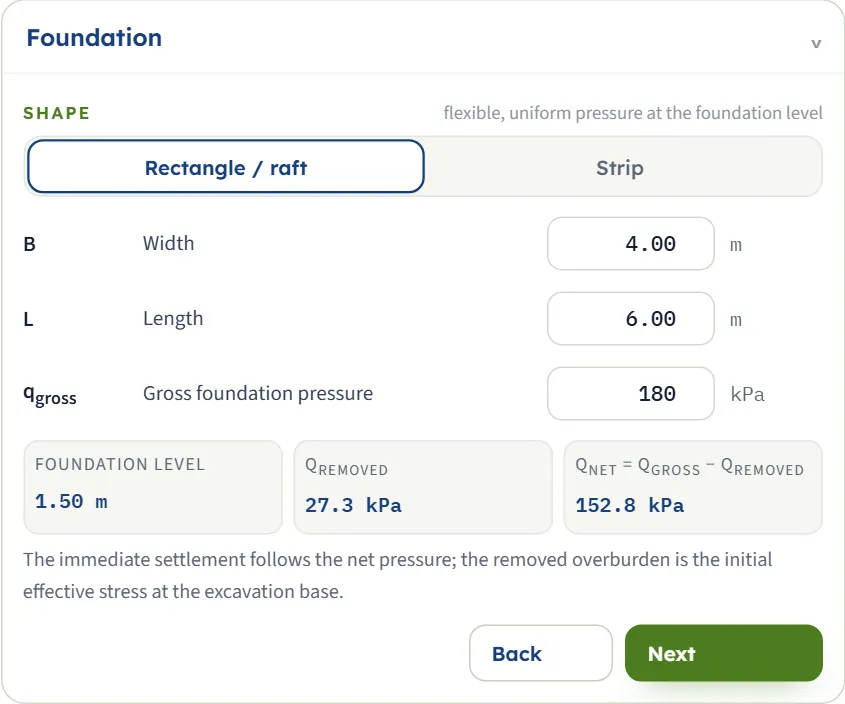
- Excavation: No puts the foundation at the ground surface; Yes takes the overburden of the excavation off the gross pressure.
- Foundation: Rectangle / raft or Strip. A strip has no length box. The water table acts only through the overburden removed by the excavation.
- Under the boxes three read-only values show the Foundation level, qremoved (the effective vertical stress at the excavation base) and qnet = qgross − qremoved.
- A box left empty keeps its previous value; a value below the limit is raised to it (a width of 0.05 m becomes 0.10 m).
| Field (unit) | Default | Range |
|---|---|---|
| zw Groundwater depth m · ft | 2.50 | 0 or more |
| Dexc Excavation depth, the foundation level m · ft | 1.50 (Yes) | 0 or more |
| B Width m · ft | 4.00 | 0.1 or more |
| L Length (rectangle only) m · ft | 6.00 | 0.1 or more |
| qgross Gross foundation pressure kPa · t/m² · ksf | 180 | 0 or more |
Analysis Settings
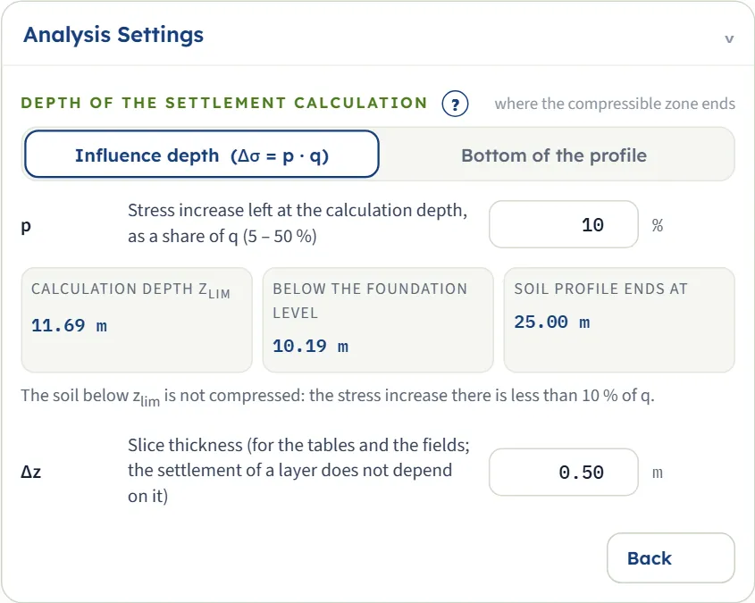
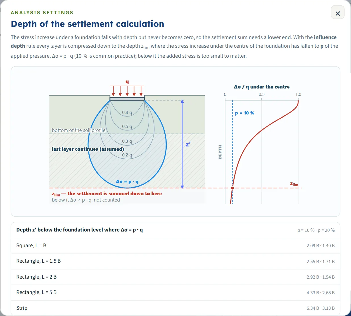
Here you choose the lower end of the settlement sum. Influence depth (Δσ = p · q) sums down to zlim, the depth where the stress increase under the centre has fallen to p of q. Bottom of the profile sums to the bottom of the last layer, as if a rigid base lay right below it. The (?) opens a sketch and a table of the depth z′ below the foundation level for typical shapes. Three read-only values show zlim, the depth below the foundation level and the depth where the profile ends, with a note that explains the case.
Δz sets the slices used for the tables and the fields. The settlement of a layer does not depend on it: 0.25, 0.50 and 1.00 m all give 24.1, 24.1 and 24.1 mm at the centre.
| Field (unit) | Default | Range |
|---|---|---|
| p stress increase left, as a share of q % | 10 | 5 to 50 (3 becomes 5, 60 becomes 50) |
| Δz slice thickness m · ft | 0.50 | 0.05 to 2 |
Choosing the calculation depth and the foundation shape
The stress increase under a foundation falls with depth but never reaches zero, so the sum needs a lower end. There are two choices.
- Influence depth (Δσ = p · q) (the starting rule). Use it when the granular soil continues well below the foundation. zlim = Dexc + z′, where z′ is the depth below the foundation level at which Δσz = p · q under the centre. Layers below zlim are not compressed. If the profile ends above zlim, the last layer is taken to continue with the same properties.
- Bottom of the profile. Use it when a rigid stratum (rock, very dense gravel) lies right below the last layer. The settlement stops at the bottom of the profile whatever the stress increase there; the module states what share of q is still left.
For the example, with p = 10 %, z′ = 10.19 m and zlim = 11.69 m, inside the medium dense sand. The dense gravelly sand below is not compressed. A smaller p goes deeper and a larger one stops sooner: p = 5 % gives zlim = 16.28 m and 24.9 mm, p = 20 % gives 8.32 m and 21.9 mm, p = 50 % gives 4.99 m and 17.2 mm. The bottom of the profile gives 25.5 mm over 25.00 m.
A profile shorter than the influence depth
A strip loads the soil to a much greater depth. The same profile with a strip of width 4 m gives zlim = 26.86 m, below the 25.00 m where the profile ends. The Analysis Settings note then reads “The soil profile ends above zlim: Gravelly sand is taken to continue from 25.00 to 26.86 m with the same properties. Choose Bottom of the profile when a rigid stratum lies below it.” The Section and Settlement views draw a line “profile ends at 25.00 m — the last layer continues (assumed)”, and the Results table marks the layer “continued from 25.00 to 26.86 m (assumed)”.
Rectangle or strip
Choose Strip for a long wall footing or embankment foundation where the length is many times the width; the length is then not used and the module gives the settlement at the edge instead of the corner. For a rectangle the corner and the centre differ by the “differential” settlement shown in the Results. With the other inputs of the example the strip gives 31.5 mm at the centre and 21.2 mm at the edge.
The excavation and the net pressure
With an excavation the foundation level is Dexc and the load that settles the soil is the net pressure qnet = qgross − qremoved, where qremoved is the effective vertical stress at the excavation base. The module takes one modulus for unloading and reloading, so the rebound of the excavation and its recovery cancel. For the example qremoved = 18.0 × 1.0 + 18.5 × 0.5 = 27.25 kPa (above the water table) and qnet = 152.75 kPa. Layers that lie wholly above the foundation level only contribute their weight. The water table matters when it lies above the excavation base: zw = 0.5 m gives qnet = 161.6 kPa and 25.4 mm; zw = 10 m leaves the example unchanged at 24.1 mm.
Analyze and read the results
Press Analyze. The bar counts four short steps (net pressure, calculation depth, Steinbrenner factors, layer settlements) and then reads Analysed — 2 layers, 21 slices down to 11.69 m with “The inputs are locked. Edit inputs clears the results; the unit system can still be changed.” The bar then has Warnings (0) and Edit inputs. When the run carries a caution, the bar adds “— 1 warning” and the Warnings window opens by itself (see Messages). The Results tab shows three cards, a line of pressures, the table by layer and the table by slice.
| Card | What it is | Example |
|---|---|---|
| Centre — flexible foundation | Settlement under the centre of a perfectly flexible foundation. | +24.1 mm |
| Corner — flexible foundation (Edge for a strip) | Settlement at the corner, with the differential settlement centre − corner. | +8.3 mm; differential +15.8 |
| Rigid foundation | A rigid foundation settles about 0.93 times the flexible centre. | +22.4 mm |
Under the cards a line gives qgross, qremoved, qnet, the foundation level and the calculation depth. The layer table lists, for each compressed layer, its type, the thickness H that is compressed, E′, ν′, the settlement at the centre and at the corner and the share of the total. Notes under a layer say how much of it was removed by the excavation, that it was compressed only down to zlim, or that it was continued below the profile.
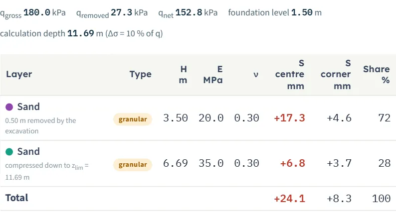
Below it Slice by slice lists every slice with its depth, layer, Δσz, εz and the settlement at the centre; tick All columns to add the thickness, E′, ν′ and the corner settlement. Click a row to open its step-by-step working in the Calculations tab.
Units and the sign of the settlement
- The unit selector in the header switches the boxes, the tables, the cards and the working between SI · kN, SI · tf and US without a new run. The drawings stay in SI (m, kPa, MPa, mm) and say so in the corner. Values you typed are kept unrounded behind the boxes: in SI · tf the unit weights show three decimals (18.0 kN/m³ shows 1.835 t/m³).
- The Sign selector beside it chooses Sign: settlement + (the default) or Sign: settlement − (the vertical displacement positive upward). The cards, tables, drawings and report then show settlement as negative: -24.1 mm in place of +24.1. The step-by-step working keeps the classical convention. Strains and stresses keep compression positive.
- The first card shows the centre; a net pressure that does not exceed the removed overburden gives a negative value, an elastic rebound.
The Calculations tab, the report and the Theory tab
The Calculations tab writes out the working of one slice, chosen in the Slice box at the top (or by clicking a row of the Results). It has five steps; steps 1, 2, 3 and 5 are open and step 4 opens on a click.
- Net pressure at the foundation level — qremoved and qnet = qgross − qremoved with your numbers (27.25 and 152.75 kPa in the example).
- The slice — its depths, the type of soil, E′ and ν, and its depths z′ below the foundation level.
- Settlement of the slice under the centre — the shape factor Is = F1 + (1 − 2ν)/(1 − ν) · F2 at the top and at the bottom of the slice, with the intermediate terms, and ΔS = qnet · α · B′ · (1 − ν²)/E · (Is bottom − Is top).
- Corner (or Edge of a strip) — the same with α = 1 (or 2) and B′ = B.
- Layer and total — the calculation depth, the settlement of the layer and the totals at the centre, at the corner and for the rigid foundation.
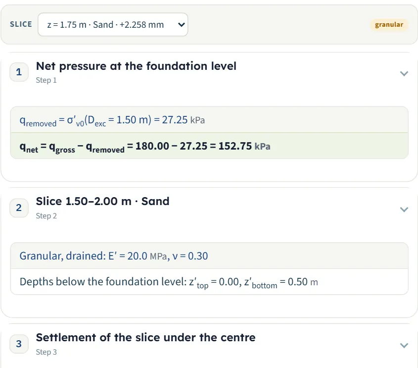
Before Analyze the tab says “Press Analyze on the Model tab first.” The working is yours to check: for the first slice of the example, B′ = 2.00 m, m′ = 1.500 and n′ = 0.250 at the bottom give Is = 0.0406, so ΔS = 152.75 × 4 × 2.00 × (1 − 0.30²)/20 000 × 0.0406 = 2.258 mm.
The report
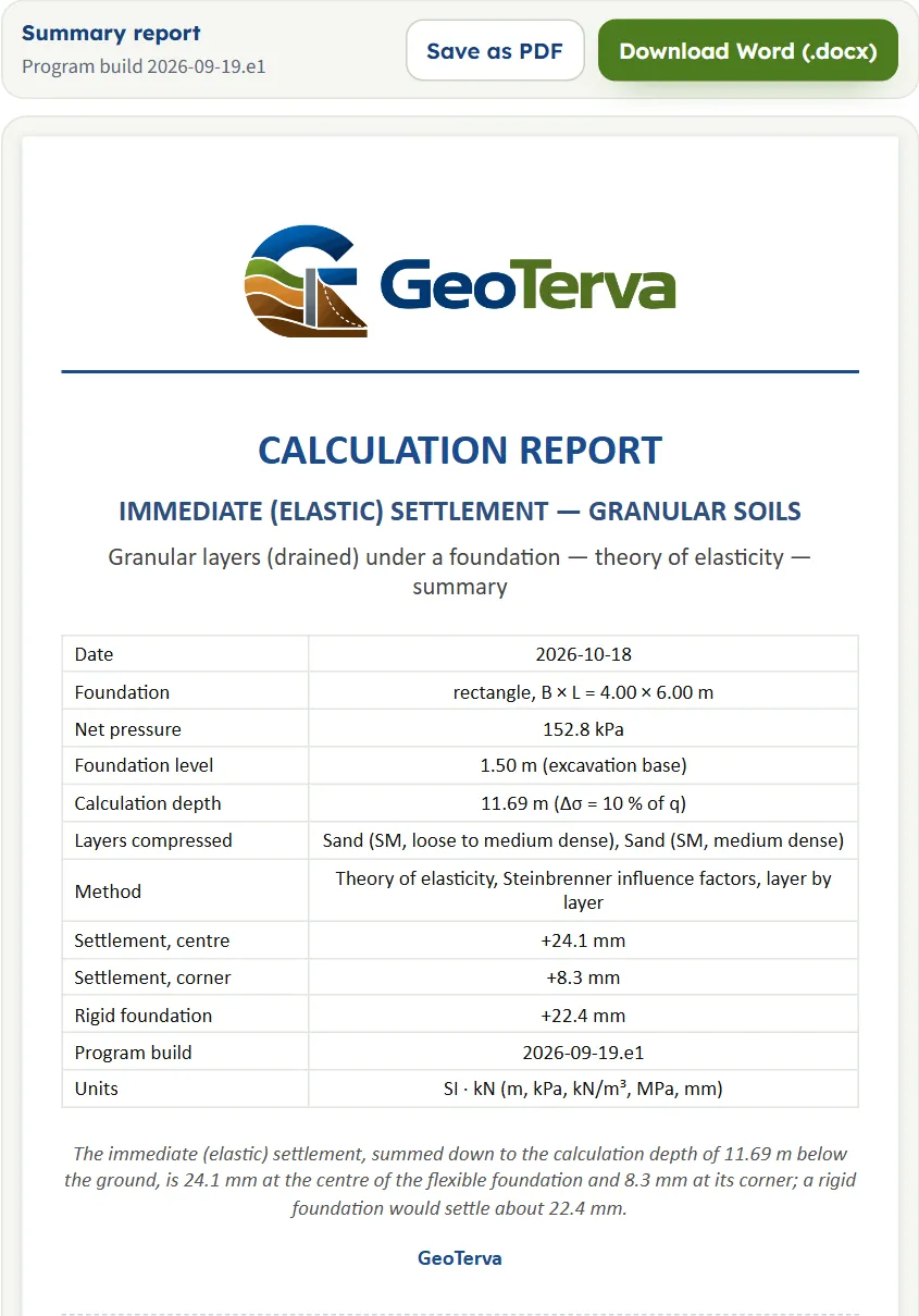
In the Report tab fill in the cover: project, location, client, report number, date (today by default), prepared by, title and qualification, checked by and optional notes. The cover is kept in the browser and saved with the model file. After Analyze the Save as PDF and Download Word (.docx) buttons are active and the report appears below; before it they are greyed and the tab says to press Analyze.
The report has eight parts: 1 Introduction and scope, 2 Soil profile and elastic parameters, 3 Foundation, loading and calculation depth, 4 Method and assumptions, 5 Immediate settlement, 6 Slice by slice, 7 Summary and 8 References. When the run carries a caution a part 7 Warnings is added and the last two become 8 and 9. It carries the section, the stress-increase field and the settlement field as figures and states the units with the conversion constants.
The Theory tab has thirteen sections: Scope, Theory of elasticity, Steinbrenner’s influence factors, Layered profile, Granular layers, Net pressure, Depth of the settlement calculation, Flexible and rigid foundations, Embedment, Colour-band fields, Sign convention and assumptions, Outside the scope, and References.
Worked example: the module’s own example
The module opens on this example the first time, and Reset to defaults brings it back.
| Section | Value |
|---|---|
| Foundation | Rectangle B = 4 m, L = 6 m, qgross = 180 kPa |
| Excavation, water table | Dexc = 1.5 m, zw = 2.5 m |
| Layers | Fill 0–1 m (E′ 8 MPa); sand 1–5 m (20 MPa); sand 5–12 m (35 MPa); gravelly sand 12–25 m (70 MPa); every ν′ = 0.30; unit weights as in the section |
| Calculation depth | Influence depth, p = 10 % |
Step 1: the net pressure
The fill (0–1 m, 18.0 kN/m³) and the first half metre of the sand above the water table (18.5 kN/m³) are removed: qremoved = 18.0 × 1.0 + 18.5 × 0.5 = 27.25 kPa, so qnet = 180.00 − 27.25 = 152.75 kPa.
Step 2: the calculation depth
For a 4 × 6 m rectangle the stress increase under the centre falls to 10 % of q at z′ = 10.19 m below the foundation level, so zlim = 1.50 + 10.19 = 11.69 m. The dense gravelly sand lies below it and is not compressed.
Step 3: the slices and the layers
The sand of 1.50–5.00 m is compressed over 3.50 m in seven slices of 0.5 m, the medium dense sand from 5.00 m to 11.69 m over 6.69 m in fourteen: 21 slices. The first slice has ΔS = 2.258 mm (see the Calculations tab), the sum of the first layer is +17.3 mm and of the second +6.8 mm.
Step 4: the totals
The settlement is checked independently by summing the Steinbrenner factors of every slice and by integrating the Boussinesq strains numerically over the loaded area; both agree with these figures (the numerical integration to within 1 %).
The same model in the other unit systems
In SI · tf the module shows qgross = 18.4 t/m², qremoved = 2.8 t/m², qnet = 15.6 t/m², E′ = 204 and 357 kg/cm² and the same 24.1 mm, 8.3 mm and 22.4 mm. In US it shows 13.12 ft × 19.69 ft, qgross = 3.76 ksf, qnet = 3.19 ksf, E′ = 418 and 731 ksf, and the settlement 0.95 in at the centre, 0.33 in at the corner and 0.88 in rigid, which is 24.1 / 25.4 = 0.95 in by hand.
How each input changes the answer
Each row changes one thing in the example (rectangle 4 × 6 m, qgross = 180 kPa, Dexc = 1.5 m, zw = 2.5 m, layers as above with γ and γsat as in the section, p = 10 %) and runs the module again. Values are settlements in mm from the Results tab: the centre and the corner (the edge for the strip) in the second column, the rigid foundation in the third.
| Change | Centre · corner | Rigid |
|---|---|---|
| The example rectangle 4 × 6 m, qgross = 180 kPa, Dexc = 1.5 m | 24.1 · 8.3 | 22.4 |
| B = 3 m a narrower foundation settles less and the calculation depth is 10.26 m | 20.9 · 7.2 | 19.4 |
| B = 6 m wider: deeper influence, 14.02 m | 28.0 · 9.4 | 26.0 |
| L = 4 m (square) shorter | 20.9 · 7.2 | 19.4 |
| L = 12 m longer | 27.8 · 9.3 | 25.8 |
| Strip, B = 4 m the last layer continues to 26.86 m; corner column is the edge | 31.5 · 21.2 | 29.3 |
| qgross = 120 kPa qnet = 92.8 kPa | 14.6 · 5.0 | 13.6 |
| qgross = 240 kPa qnet = 212.8 kPa | 33.5 · 11.5 | 31.2 |
| No excavation qnet = 180 kPa, foundation at the surface, 10.19 m | 39.4 · 12.7 | 36.6 |
| Dexc = 3 m qnet = 129.4 kPa | 17.7 · 6.0 | 16.4 |
| zw = 0.5 m more overburden removed: qnet = 161.6 kPa, so more settlement | 25.4 · 8.7 | 23.7 |
| E′ of layer 2 = 10 MPa was 20 | 41.3 · 12.8 | 38.4 |
| E′ of layer 2 = 40 MPa was 20 | 15.4 · 6.0 | 14.3 |
| E′ of layer 3 = 70 MPa was 35 | 20.7 · 6.4 | 19.2 |
| ν′ = 0.20 in layers 2 and 3 was 0.30 | 26.0 · 9.2 | 24.2 |
| ν′ = 0.40 in layers 2 and 3 was 0.30 | 21.4 · 7.1 | 19.9 |
| Bottom of the profile rigid base at 25.00 m | 25.5 · 9.5 | 23.7 |
| p = 5 % zlim = 16.28 m | 24.9 · 8.9 | 23.1 |
| p = 20 % zlim = 8.32 m | 21.9 · 6.8 | 20.4 |
- The modulus: the settlement is inversely proportional to E′ layer by layer, so halving E′ of the upper sand from 20 to 10 MPa raises the centre settlement from 24.1 to 41.3 mm, and the stiffness of the upper layers counts more because the strains are largest there.
- ν′ acts through the lateral stresses: a larger value gives a smaller settlement here.
- The excavation reduces the net pressure, and so the settlement; a deeper excavation also moves zlim down.
- The water table changes the answer only when it lies above the excavation base; at 10 m it equals the example, at 0.5 m it raises qnet.
- The unit weight of a layer above the foundation level enters through qremoved: γ = 22 kN/m³ in the fill gives qnet = 148.8 kPa and 23.4 mm.
- The depth rule: the settlement grows only slowly beyond p = 10 %, as the added strains are small: 24.1 mm at 10 % and 24.9 mm at 5 %.
Messages: stops and cautions
When the module stops
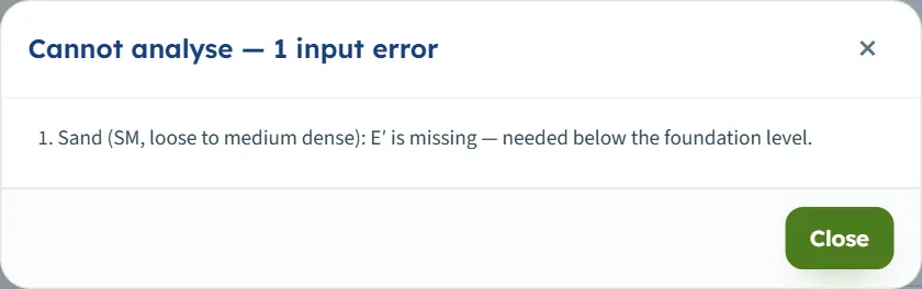
The module needs a modulus and a Poisson’s ratio for every layer that will be compressed. When one is missing the analysis stops and nothing is calculated: a window Cannot analyse — 1 input error (or “… N input errors”) lists the problems, the bar stays Not analysed, and the inputs stay editable.
| Cause | Message |
|---|---|
| E′ empty, zero or negative in a compressed layer | “Sand (SM, loose to medium dense): E′ is missing — needed below the foundation level.” (the layer’s own name comes first) |
| ν′ empty in a compressed layer | “Sand (SM, loose to medium dense): ν must be at least 0 and below 0.5 for a granular layer.” |
Most other boxes cannot be left wrong: a box left empty returns to its old value and a value outside its range is moved to the limit (see the tables in the model sections).
Cautions
A caution does not stop the run. The Warnings window opens after Analyze with the caution and, below it, the assumptions of the analysis; a bar with the first caution appears at the top of the Results and Report tabs, and the report gets a part Warnings. Warnings (n) in the Analyze bar reopens the window.
| Cause | Message |
|---|---|
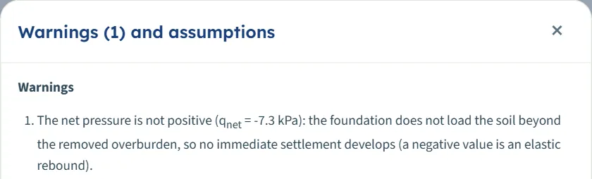
| qgross not larger than qremoved (-1.1 mm for qgross = 20 kPa) | “The net pressure is not positive (qnet = -7.3 kPa): the foundation does not load the soil beyond the removed overburden, so no immediate settlement develops (a negative value is an elastic rebound).” |
| The excavation is deeper than the profile | “The excavation reaches the bottom of the soil profile (25.00 m).” (together with the net-pressure caution) |
Notes that are not cautions
- “The soil below zlim is not compressed: the stress increase there is less than 10 % of q.” — the normal case of the influence-depth rule.
- The profile that ends above zlim, described above, and the rigid-base note of Bottom of the profile: “A rigid base is assumed right below the profile; the stress increase at its top is still n % of q.”
Good practice and common mistakes
- Put the effort into E′. The settlement is inversely proportional to it layer by layer. Split a thick layer when the stiffness grows with depth, and give each layer the value that suits its depth.
- Use this module for drained granular soil only. A clay layer settles undrained and consolidates later; use the cohesive and the consolidation modules, or Settlement 2D for the total.
- Read the net pressure. qgross is the pressure at the foundation level; the excavation takes qremoved off it. Check that the foundation level you give is the excavation depth.
- Check where the profile ends. If the influence depth lies below it, the last layer is taken to continue with the same properties. Choose Bottom of the profile only when a rigid stratum really lies there.
- Rectangle or strip. A footing long compared with its width is a strip; use the rectangle for a pad and the strip for a wall.
- Flexible or rigid. The centre and the corner of the flexible foundation bracket the behaviour of a real footing; the rigid value is 0.93 times the centre.
- No embedment correction is applied (the factor is taken as 1), a choice that errs on the safe side.
- Remember the model is kept in the browser. Use Save to file… to keep it with the project, and Reset to defaults to start again from the example.
- Mind the sign. In the minus convention settlements show as negative numbers.
Frequently asked questions
What does this module calculate?
The immediate settlement of a flexible rectangular or strip foundation on sand and gravel layers that settle drained, by the theory of elasticity with Steinbrenner’s influence factors, layer by layer. For the example it gives 24.1 mm at the centre, 8.3 mm at the corner and 22.4 mm for a rigid foundation.
Why is there no consolidation for sand and gravel?
Granular soil is permeable, so the water leaves as fast as the load is applied and the soil settles as the load arrives, with the drained modulus E′ and ν′. Clay layers consolidate over time; see the Consolidation settlement module.
What are the centre, corner and rigid settlements?
The centre is the settlement under the middle of a perfectly flexible foundation, the corner (the edge of a strip) is the settlement at its corner, and a rigid foundation settles about 0.93 times the flexible centre.
How is the calculation depth chosen?
By the influence-depth rule it is the depth zlim where the stress increase under the centre has fallen to p of the applied pressure (5 to 50 %, 10 % by default). Alternatively the sum stops at the bottom of the profile, with a rigid base below it.
What if my profile is shorter than the influence depth?
With the influence-depth rule the last layer is taken to continue with the same properties down to zlim, and the module says so in the notes, the drawings and the Results table. Choose Bottom of the profile when a rigid stratum lies right below the profile.
What is the net pressure?
The gross pressure minus the effective vertical stress that the excavation removes at the foundation level. With the example, 180 − 27.25 = 152.75 kPa.
Does the slice thickness change the settlement?
No. It only sets the slices of the tables and the colour fields; 0.25, 0.5 and 1 m all give the same total.
Can I drag or zoom the drawing?
No. The drawings show the model and follow the boxes; you change the model in the Model tab. After Analyze the inputs are locked until you press Edit inputs.
Does the module remember my inputs?
Yes. Every change is kept in this browser and the page opens again on the model you last worked on, analysed or not, together with the unit system and the sign convention. Save to file, Open file and Quick Save keep versions; Reset to defaults brings the example back.
Which units can I use?
SI · kN, SI · tf and US, switchable at any time, even after Analyze. The drawings stay in SI.
Why does the settlement appear negative?
Either you chose the sign convention “settlement −”, or the net pressure is not positive and the soil rebounds; the second case comes with a warning.
What does the report contain?
A cover with your project details, then the introduction, the soil profile, the foundation and the calculation depth, the method and assumptions, the settlement by layer with the figures, the slice table, the summary and the references (and a Warnings part when there is one). It is saved as PDF or Word after Analyze.