

What the module calculates
Consolidation settlement gives the primary consolidation settlement of clay layers under a rectangular (raft) or strip foundation, and how fast it develops. It follows every slice of clay along its stress path: the initial stress, the unloading and swelling when you excavate to the foundation level, the reloading back to the initial stress, the recompression up to the preconsolidation pressure σ′p and the virgin compression beyond it. The settlement is summed slice by slice down to a calculation depth, and Terzaghi’s theory gives the settlement against time.
Sb is the reloading along the swelling line (Cs) back to σ′v0, Sr is the recompression (Cr) from σ′v0 up to σ′p, and Sv is the virgin compression (Cc) beyond σ′p. Settlement is positive and heave negative unless you change the sign in the header.
What you can describe
- A profile of clay layers from the ground surface down, each with its unit weights, its compressibility (e0, Cc, Cr, Cs or mv), its Cv, its OCR or laboratory σ′p, and one or two-way drainage.
- A water table, hydrostatic below it and unchanged by the excavation.
- An excavation to the foundation level, with its own plan if it differs from the foundation, and the choice of where the settlement is measured from.
- A rectangular or strip foundation with its gross pressure at the foundation level.
- The calculation depth: the influence depth, where the stress increase has fallen to a share p of q, or the bottom of the profile.
The module gives the heave, the settlement of every layer and of the foundation, the stress path of every slice, the settlement–time curve with t50 and t90, and colour bands of stress, strain and settlement over the whole section. It writes out the working and prepares a PDF or Word report.
What belongs to other modules
- Clay layers only. The module has no granular layer. The immediate (elastic) settlement belongs to Elastic settlement, cohesive and Elastic settlement, granular; Settlement 2D adds the two over a profile of both kinds of layer.
- The stress increase is the Boussinesq stress under the centre of the foundation. The stress under other points, loads of other shapes and their charts are in the Stresses in a soil mass modules.
- The module gives the settlement, not the bearing capacity: for that, see the Bearing capacity modules.
Before you start: what you need
Have these ready from your investigation and design:
- The soil profile (boreholes): layer depths from the ground surface, without gaps; the unit weight γ above the water table and γsat below it.
- e0, Cc, Cr, and Cs if you have it (oedometer tests): for the e – log σ′ method. Cs is the swelling index; left empty, Cs = Cr is used.
- Or mv (oedometer tests): for the mv method, a single linear coefficient.
- OCR, or σ′p of each layer (oedometer tests, stress history): the preconsolidation pressure, as OCR or as a laboratory value (one definition for the whole model).
- Cv of each layer, and the drainage (oedometer tests, the stratigraphy): only for the settlement–time curve. Double drainage uses H/2 as the drainage path, single uses H.
- The water table depth zw (boreholes, piezometers): below the ground surface; it is not changed by the excavation.
- The excavation depth Dexc (your design): the foundation level. Zero, or “No”, puts the foundation at the ground surface.
- The foundation B, L, qgross (your design): width, length (not for a strip) and the gross pressure at the foundation level.
Quick start in seven steps
- Open the module and choose the units
Open Consolidation settlement from the Settlement family. Pick SI · kN, SI · tf or US in the header; you can change it at any time, even after Analyze. The sign selector beside it chooses settlement + or settlement −.
- Describe the soil
In Soil profile give the depth to the bottom of each layer, its name and its unit weights. Press Next and, in Compressibility, fill one row per layer. Enter the water table in Groundwater.
- Describe the excavation
In Excavation choose Yes or No, give Dexc, and pick the plan and where the settlement is measured from.
- Describe the foundation
In Foundation pick Rectangle / raft or Strip and enter B, L and qgross. The three read-outs under the boxes give the foundation level, qremoved and qnet.
- Choose the analysis
In Analysis Settings choose the compressibility method, the definition of σ′p, the calculation depth, the slice thickness Δz and whether you want the settlement–time curve.
- Press Analyze
Press Analyze at the foot of the Model tab. The bar reads Analysed, the inputs lock, and the drawing switches to the Contours view.
- Read the results and take the report
The Results tab gives the heave, the settlement and the table by layer and by slice; Calculations writes out any slice; Report saves a PDF or a Word file.
The screen: five views of the section
The layout is the one every GeoTerva module shares, described in the workspace guide. The drawing on the left has five views, chosen with the buttons above it; the Model, Results, Calculations, Report and Theory tabs are on the right. Every view has a bar of chips above it; the chips only change what is drawn, never the calculation.
- Section is the soil profile with the water table, the excavation, the foundation, its load and the calculation slices on the vertical through the centre. It follows the inputs live, before Analyze. After Analyze it adds the heave, the settlement and the net value to the title. Chips: Slices, Dimensions, Layer labels.
- Contours paints a field over the whole section as 36 equal colour bands with a legend. The Field chips are σv, u, σ′v0, σ′p, Δσexc, Δσload, σ′exc, σ′final (the default), εv and S; the other chips are Foundation and Layer labels.
- Stresses plots the vertical stresses on the centre line against depth, with the stress changes beside them. Seven chips switch the curves: σv, u, σ′v0, σ′p, σ′exc, σ′final and the net change.
- Settlement paints the settlement of a point at each depth with a trough drawn over the foundation, and a bar for every slice (heave, Cs back, Cr, Cc). Field chips: Strain εv, Settlement S (the default), Heave, Net; other chips: Trough, Labels, Slice bars.
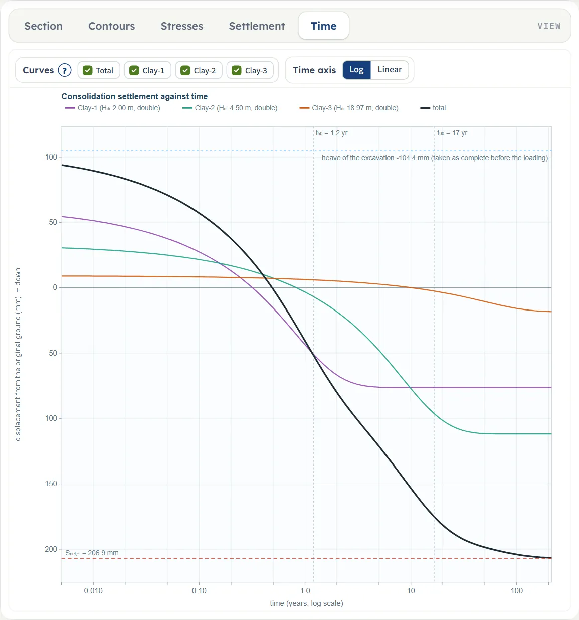
- Time plots the settlement against time for the whole profile and for each layer. Chips: Total and one per layer, and a Log or Linear time axis.
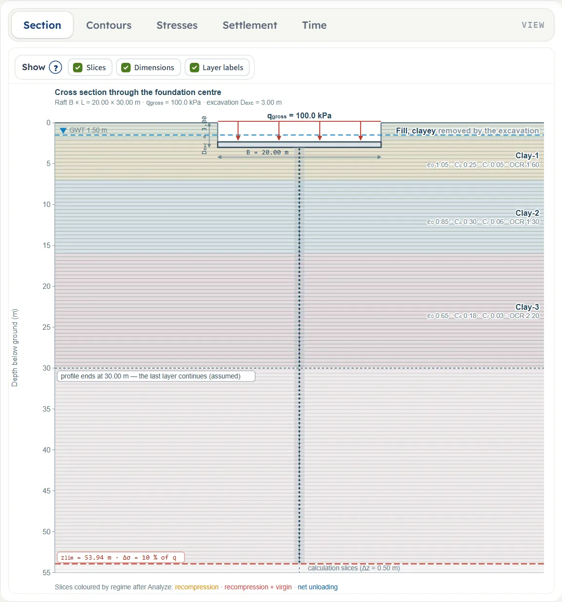
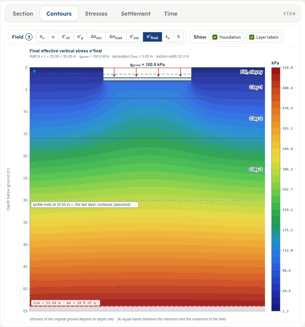
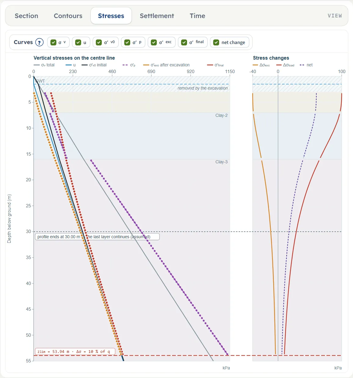
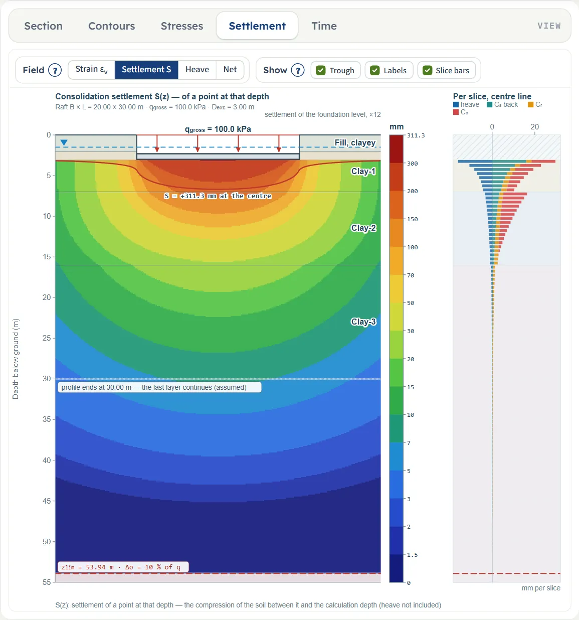
Before and after Analyze
The page opens on the Contours view, which has nothing to paint yet: it shows the layers and the words “Press Analyze”. The Section view follows your inputs while you edit. After Analyze the drawing switches to Contours; after Edit inputs it returns to Section. When the page opens again on a model you saved, it starts on Section, or on Contours if that model was analysed.

Entering the model, section by section
The Model tab has a Model data card and six sections. The sections work as a walk-through: one is open at a time, and Back and Next at the foot of each move to the neighbour; clicking a title opens that section and closes the other. Analyze waits below the last one. The tables give the unit in SI · kN first; SI · tf and US show the same values converted, for example 100 kPa is 10.2 t/m² and 2.09 ksf. Defaults are the example project.
Model data
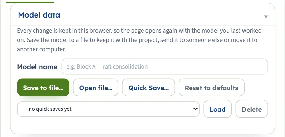
This card keeps your work. Model name labels it. Save to file… writes a .gtrv file and Open file… reads one back. Quick Save… asks for a name and keeps this version in the browser; choose it in the list and press Load to come back to it, Delete removes it. Reset to defaults returns to the example. A line under the buttons reports what happened. Every change is also kept automatically: the page opens again on the model you last worked on, analysed or not.
Soil profile
One row per layer from the ground surface down. From is read-only: it is the bottom of the layer above (0 for the first). Type the bottom of each layer in To; the next layer starts there. A value at or above the top of the layer is ignored. + Add layer appends a layer 2 m thick below the last one, and × deletes a layer (the last remaining layer cannot be deleted). Nothing in the profile can be edited after Analyze until you press Edit inputs.
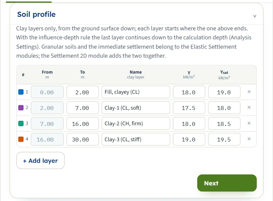
| Column | Default of the four layers |
|---|---|
| To (m · ft) | 2.00 · 7.00 · 16.00 · 30.00 |
| Name | Fill, clayey (CL) · Clay-1 (CL, soft) · Clay-2 (CH, firm) · Clay-3 (CL, stiff) |
| γ (kN/m³ · t/m³ · pcf) | 18.0 · 17.5 · 18.0 · 19.0 |
| γsat (same units) | 19.0 · 18.0 · 18.5 · 19.5 |
| A new layer (+ Add layer) | Clay-5 (the number follows the layers present), γ 18.5, γsat 19.0, e0 0.9, Cc 0.3, Cr 0.05, Cs empty, mv 0.0003 1/kPa, Cv 1 m²/yr, OCR 1.2, σ′p 100 kPa, double drainage |
Compressibility
One row per layer. A layer, or the part of a layer, above the foundation level is removed by the excavation: its row says “Above the foundation level — removed by the excavation; only its unit weight is used.” A layer below the calculation depth says “Below the calculation depth zlim … — not compressed.” The label of the last layer shows “→” and the calculation depth when it continues down to it. Boxes the chosen method does not use are shaded: e0, Cc, Cr and Cs with the mv method, mv with the e – log σ′ method, Cv when the settlement–time curve is off.
Drainage is Double (path H/2) or Single (path H). The fill layer carries the same kind of values (it has OCR 2.0 and e0 0.80), used only if the excavation is switched off and the fill lies below the foundation level.
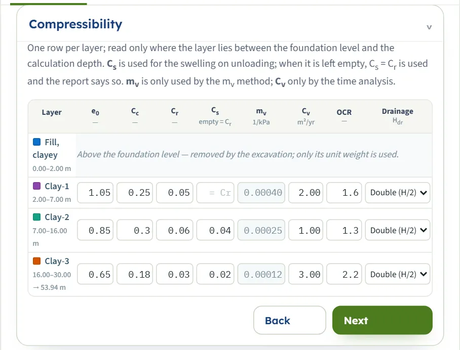
| Box | Default, Clay-1 · 2 · 3 |
|---|---|
| e0 (—) | 1.05 · 0.85 · 0.65 |
| Cc (—) | 0.25 · 0.30 · 0.18 |
| Cr (—) | 0.05 · 0.06 · 0.03 |
| Cs (—) | empty (= Cr) · 0.04 · 0.02 |
| mv (1/kPa) | 0.00040 · 0.00025 · 0.00012 |
| Cv (m²/yr · ft²/yr) | 2.00 · 1.00 · 3.00 |
| OCR (—) | 1.6 · 1.3 · 2.2 |
| σ′p (kPa), laboratory | 80 · 90 · 150 · 350 (four layers) |
| Drainage | Double · Double · Double |
Groundwater
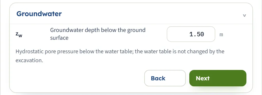
One number: the depth zw of the water table below the ground surface, default 1.50 m. Pore pressure is hydrostatic below it (γw = 9.81 kN/m³) and the excavation does not change the water table. A water table deeper than the whole profile simply means no layer is submerged.
Excavation
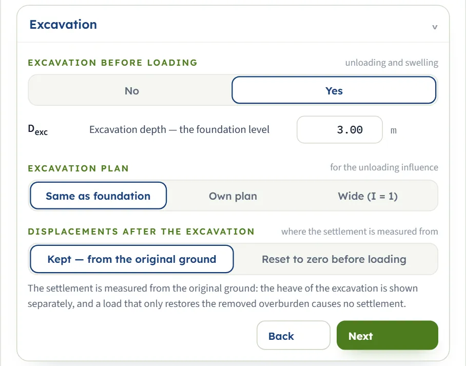
No puts the foundation at the ground surface; Yes (the default) excavates to Dexc, which is then the foundation level. The plan buttons are Same as foundation, Own plan and Wide (I = 1); the displacement buttons are Kept — from the original ground and Reset to zero before loading; the table uses their short names.
| Choice | What it does |
|---|---|
| Dexc (m · ft), default 3.00 | Excavation depth, zero or more. The stress removed is qremoved, the initial effective stress at that depth. |
| Same as foundation (default) | The unloading acts through the Boussinesq influence of the foundation’s own B × L. |
| Own plan | Two more boxes, Bexc and Lexc (the length is not asked for a strip), give a different excavation plan. They start at the foundation size. |
| Wide | The unloading acts with I = 1 at every depth, as for an excavation much wider than deep. |
| Kept (default) | The settlement is the net deformation after loading, measured from the original ground. A load that only restores the removed overburden causes no settlement. |
| Reset to zero | The settlement is measured from the heaved excavation base and includes the recompression of the heave. |
Foundation
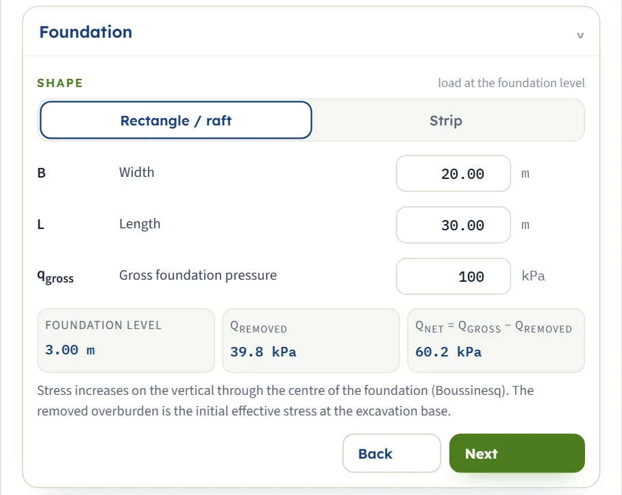
Rectangle / raft (default) or Strip. The length box disappears for a strip. Three read-outs follow the inputs: the foundation level, qremoved and qnet = qgross − qremoved. The stress increase below the foundation is computed from qgross (the excavation unloading is a separate phase), so qnet is a reading, not an input.
| Field | Default |
|---|---|
| Width B (m · ft) | 20.00; at least 0.1 |
| Length L (m · ft) | 30.00; at least 0.1; not for a strip |
| Gross pressure qgross (kPa · t/m² · ksf) | 100; zero or more |
Analysis Settings
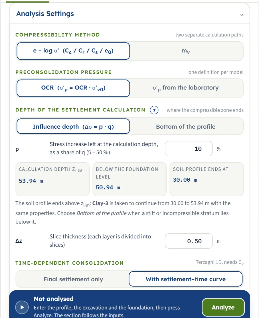
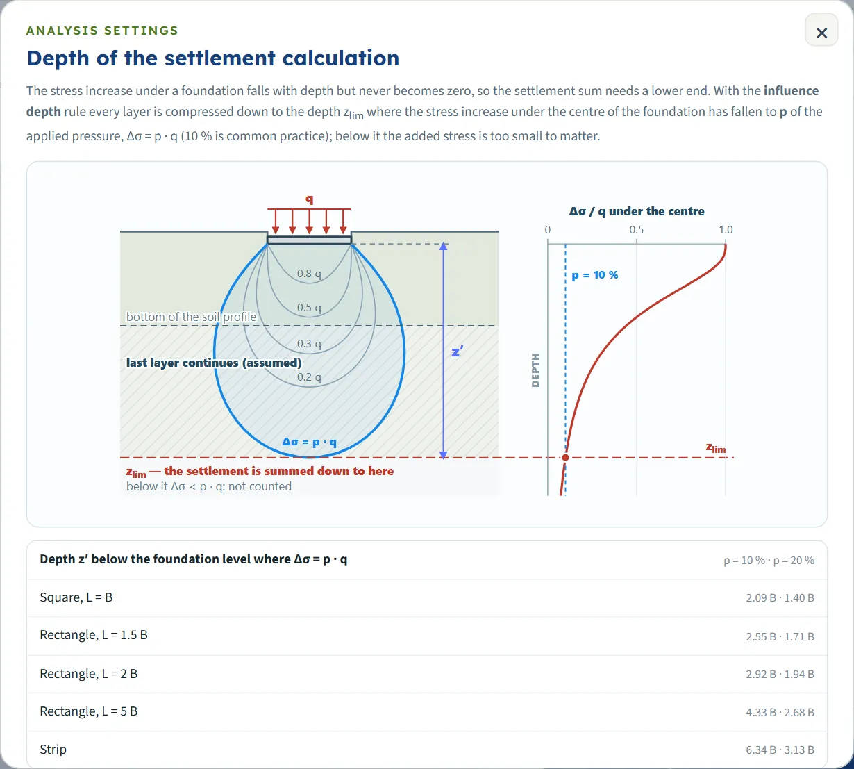
The section holds the choices that decide the method; they are described under “Choosing the method and the options” below. Its boxes: p (5 to 50 %, default 10, a value outside the range is brought back to the nearest limit), and Δz (default 0.50 m, between 0.05 and 2 m in the box). Three read-outs give the calculation depth zlim, the depth below the foundation level, and where the soil profile ends; a note says whether the last layer continues, the soil below zlim is left out, or the two coincide. The (?) beside the depth rule opens a window that explains the influence depth.
Choosing the method and the options
Six choices shape the answer. Each row of the next table is the example with only that choice changed; the numbers are those of the module, in mm, as heave / Sc.
| Choice | Heave / Sc mm | Settlement mm |
|---|---|---|
| The example | -104.4 / 311.3 | 206.9 |
| mv method | -186.4 / 468.6 | 282.2 |
| Laboratory σ′p | -104.4 / 304.8 | 200.3 |
| Profile bottom | -102.1 / 303.9 | 201.8 |
| Reset to zero | -104.4 / 311.3 | 311.3 |
| Wide plan | -131.8 / 297.8 | 166.0 |
| Strip, B = 20 m | -112.6 / 340.3 | 227.7 |
The rows in order: the example (e – log σ′, OCR, influence depth 10 %, kept from the original ground); the mv method (the mv of each layer, linear); laboratory σ′p of 80, 90, 150 and 350 kPa; a calculation depth that stops at 30.00 m; reset to zero (settlement measured from the excavation base); the wide plan (unloading with I = 1); and a strip of the same width with endless length.
e – log σ′ or mv
- e – log σ′ (Cc / Cr / Cs / e0) follows the stress path: S = C · ΔH/(1 + e0) · log10(σ′ end / σ′ start) on each branch. Use it when you have oedometer curves.
- mv is linear and has one coefficient for unloading and reloading: δH = mv · Δσ′ · ΔH. It has no σ′p and no virgin branch. With the same soil it gives 468.6 mm of loading settlement here against 311.3 mm, because one coefficient is carried over the whole range; use it with a mv measured over the stress range of the foundation.
OCR or laboratory σ′p
With OCR, σ′p = OCR · σ′v0 at every slice, so it grows with depth. With the laboratory value, each layer has one σ′p, never taken below σ′v0. Either way σ′p is the historical maximum and the excavation does not reduce it. An OCR below 1, or a laboratory σ′p below σ′v0, is replaced by σ′v0 and reported as a warning (see Messages).
The calculation depth
The stress increase never reaches zero, so the sum needs a lower end. With Influence depth (Δσ = p · q) it ends where the stress increase under the centre has fallen to p of q; for the example, p = 10 % gives zlim = 3.00 + 50.94 = 53.94 m. The profile of the example ends at 30 m, so the last layer is taken to continue down to zlim with the same properties, and the Section view, the Results table and the report say so. If the profile is deeper than zlim, the soil below it is not compressed. With Bottom of the profile the sum stops at the last layer, an incompressible stratum is assumed below it, and the stress increase left there is shown as a share of q.
The excavation and the reference of the settlement
An excavation unloads the clay, which swells (the heave). When the foundation loads it the clay first retraces its swelling line back to σ′v0; only a load above that gives a net settlement from the original ground. With Kept the settlement of the foundation is Snet = Sc + heave, 206.9 mm here, and it is reported as 0 if the net value is negative, with a note that the ground ends above its original level. With Reset, the heave is regarded as already finished before the building and the settlement is Sc, 311.3 mm, the number that answers “the excavation stayed open and heaved before the building: how much does the building settle?”. The heave itself is reported separately in both cases.
Choosing the excavation plan
Same as foundation is the usual choice. Wide unloads with I = 1 at every depth (a larger heave, -131.8 mm); Own plan lets the unloading act through another B × L, for example a basement larger than the raft (40 × 60 m gives -119.4 mm of heave, 10 × 15 m gives -84.2 mm).
Analyze and read the results
Press Analyze. After a short progress line the bar reads Analysed — 3 layers, 102 slices down to 53.94 m, the inputs are locked (“Edit inputs clears the results; the unit system can still be changed.”), a message appears for a moment (“Analysed — the colour bands show the selected field; see also Stresses, Settlement, Time and the Results tab.”) and the drawing switches to Contours. The Model tab stays on the screen; open Results for the numbers. If the run has cautions, a Warnings window opens by itself (see Messages).
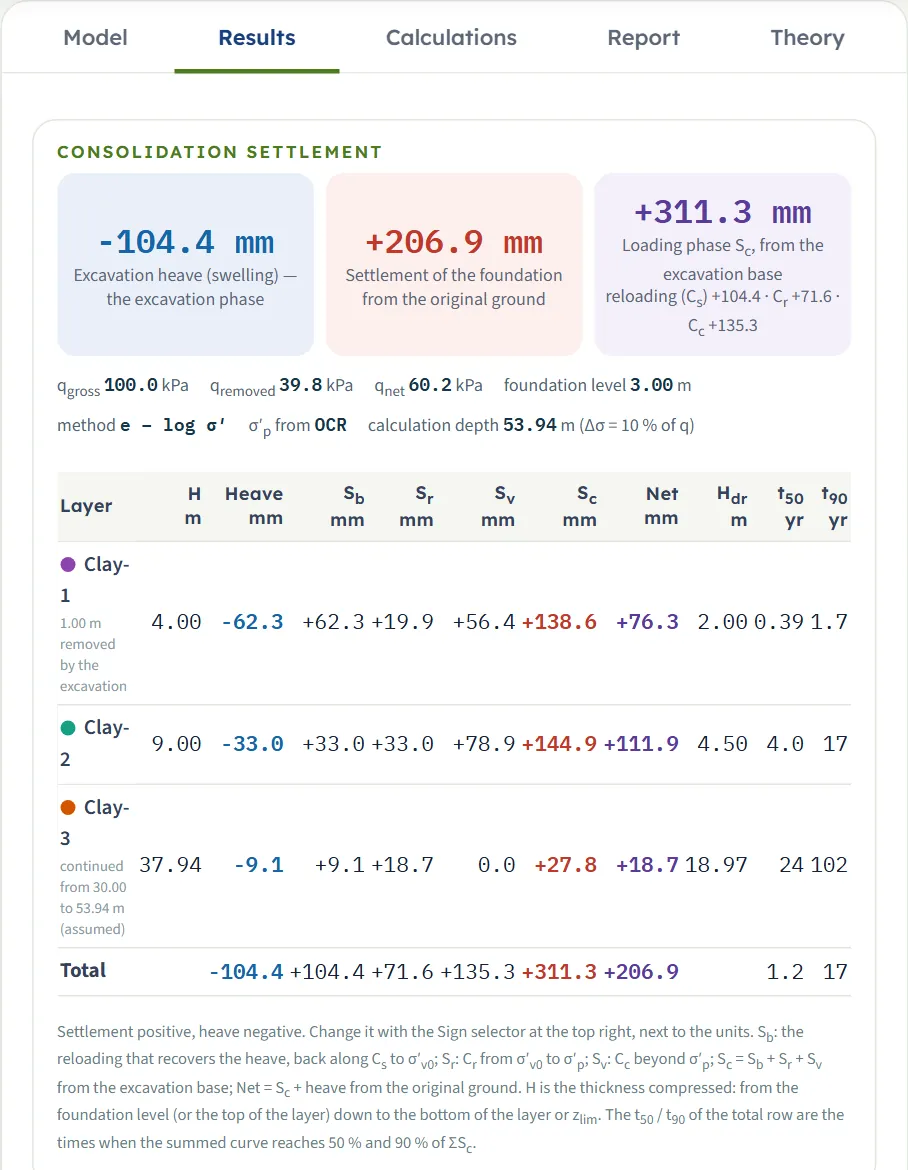
| Card | What it is | Example |
|---|---|---|
| Excavation heave (swelling) | The swelling of the clay when the excavation unloads it, negative. | -104.4 mm |
| Settlement of the foundation | From the original ground (Kept), from the excavation base (Reset), or from the ground surface (no excavation). | +206.9 mm |
| Loading phase Sc | The compression from the excavation base, with Sb, Sr and Sv written out under it (after a reset the third card shows the net value from the original ground). | +311.3 mm; reloading +104.4, Cr +71.6, Cc +135.3 |
A line under the cards gives qgross, qremoved, qnet, the foundation level, the method, the source of σ′p and the calculation depth with its rule.
The table by layer
One row per layer that is compressed, with its thickness H (from the foundation level or the top of the layer down to its bottom or zlim), the heave, Sb, Sr, Sv, Sc, the net value, and, with the time curve on, Hdr, t50 and t90. A remark under the name says when part of a layer is removed by the excavation, when the last layer continues to zlim (assumed), or when a layer is compressed only down to zlim. The Total row gives the sums and the t50 and t90 of the summed curve. The table fits the width of the panel. The note below it states the sign convention and what each column is.
| Layer | Heave / Sc mm | Net mm |
|---|---|---|
| Clay-1 H = 4.00 m, 1.00 m removed | -62.3 / +138.6 | +76.3 |
| Clay-2 H = 9.00 m | -33.0 / +144.9 | +111.9 |
| Clay-3 H = 37.94 m | -9.1 / +27.8 | +18.7 |
| Total | -104.4 / +311.3 | +206.9 |
The table by slice
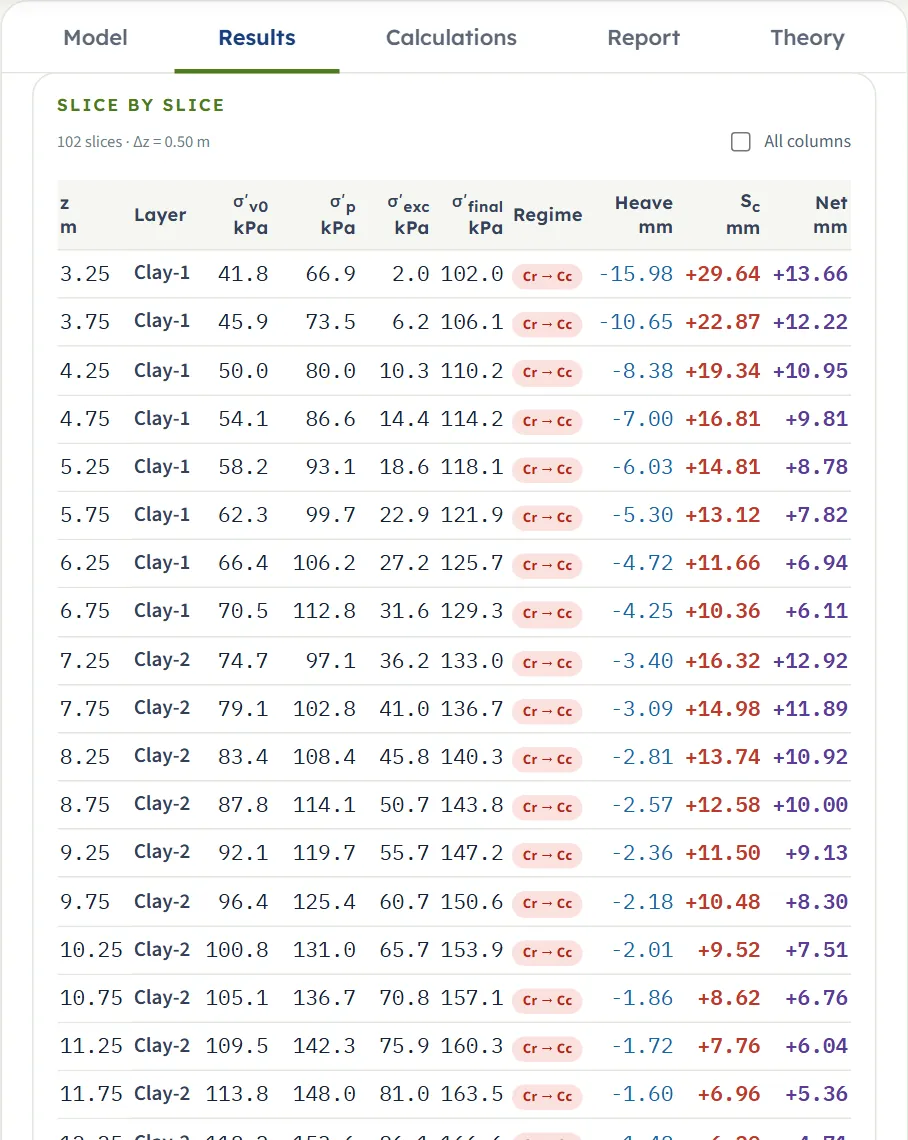
Below it, Slice by slice lists the σ′v0, σ′p, σ′exc, σ′final, the Regime of every slice (Cr → Cc, Cr only, Cc only, Cs (heave recovered), Cs (net unloading); mv with that method), the heave, Sc and the net value. All columns adds ΔH, σv0, u0, Δσexc, Δσload, Sb, Sr and Sv. A click on a row opens the working of that slice in the Calculations tab.
Using the numbers
- The settlement of the foundation is the centre value on the vertical through the centre of the foundation; the module does not give the value at the edge or the differential settlement.
- Read t50 and t90 of the Total row as the times when the summed curve reaches 50 % and 90 % of the loading settlement Sc. The heave is taken as complete before the loading.
- Changing the units or the sign after Analyze re-states the results without a new run. With Sign: settlement − every displacement changes sign (the card reads −206.9 mm); strains and stresses keep compression positive.
The Calculations tab, the report and the Theory tab
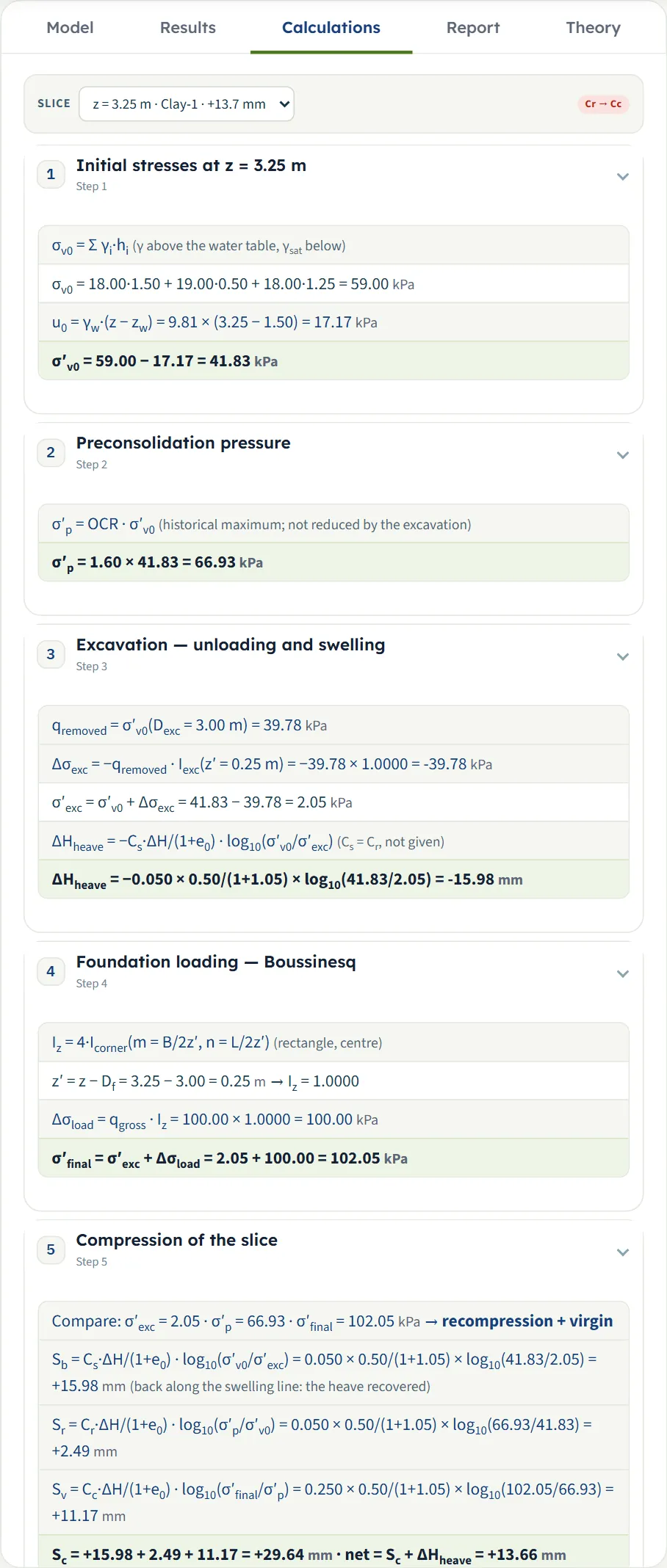
The Calculations tab writes out the working for one slice, chosen in the Slice list at the top (the list gives z, the layer and the net value of each slice; a click on a row of the slice table also opens it). The regime of the slice is shown beside the list. The steps open and close with a click:
- Initial stresses — σv0 = Σ γ·h, u0 and σ′v0 with your numbers.
- Preconsolidation pressure — σ′p = OCR · σ′v0, or the laboratory value.
- Excavation — unloading and swelling — qremoved, Δσexc, σ′exc and the heave of the slice (Excavation alone, with no heave, when there is none).
- Foundation loading — Boussinesq — the influence factor at z′ below the foundation level, Δσload and σ′final.
- Compression of the slice — the regime, then Sb, Sr, Sv and their sum; with the mv method, Sc = mv·Δσ′·ΔH.
- Layer and total — the calculation depth, the layer’s sums, the totals and the settlement of the foundation.
- Time — only with the time curve on and a Cv: Hdr, t50 and t90 of the layer and of the whole profile.
The working is always written in the classical sign (settlement +, heave −); with the other sign selected a note above it says so.
The report
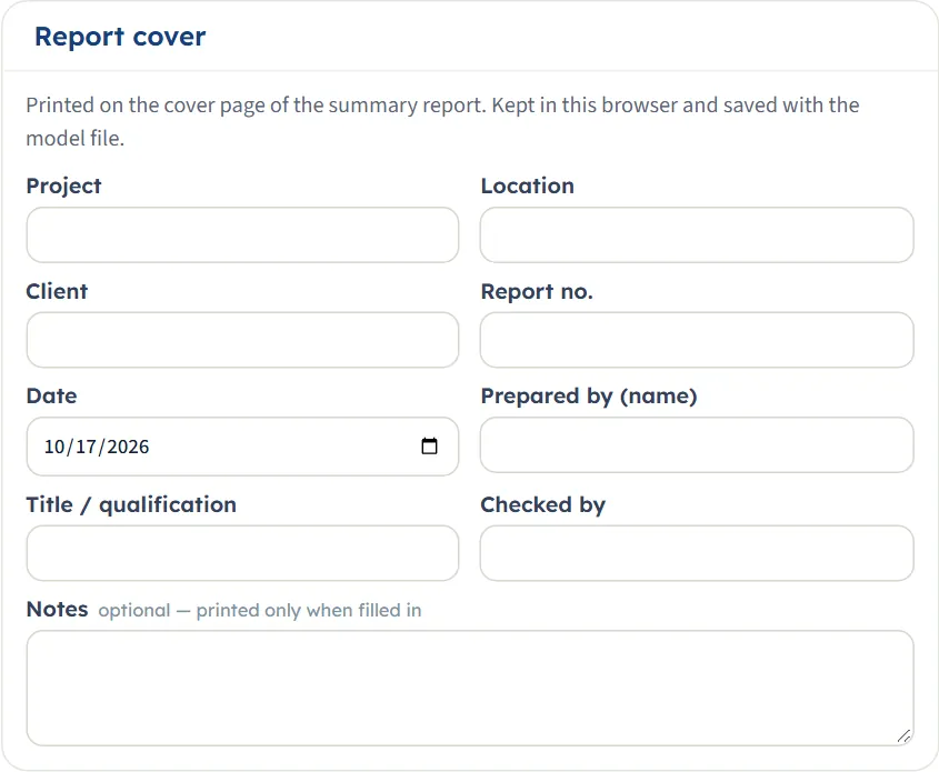
In the Report tab fill in the cover: project, location, client, report number, date, prepared by, title / qualification, checked by and optional notes. The cover is kept in this browser and saved with the model file. After Analyze, Save as PDF (the print window, where you choose “Save as PDF”) and Download Word (.docx) are available; before it they are greyed out and the tab says to press Analyze. The preview below the buttons is the report itself.
The report has eight parts: 1 Introduction and scope, 2 Soil profile and parameters, 3 Excavation, foundation and calculation depth, 4 Stress path and assumptions, 5 Consolidation settlement, 6 Slice by slice, 7 Time-dependent consolidation, 8 Summary. It carries the section, stress, settlement and time drawings and states the units. When the run carries warnings, the Report tab shows the same warning bar as the Results tab.
The Theory tab
The Theory tab has fifteen sections, each of which opens and closes: Scope, Stress path, Slices and initial stresses, Preconsolidation pressure, Excavation — unloading and swelling, Stress increase — Boussinesq, Depth of the settlement calculation, Compression regimes, Where the settlement is measured from, the mv method, Time-dependent consolidation, Colour-band fields, Sign convention and assumptions, Outside the scope, and References.
Worked example: the module’s own example
The module opens on this example, so you can follow every number on your own screen. A 20 × 30 m raft carries qgross = 100 kPa at the bottom of a 3 m excavation in four clay layers (0–2, 2–7, 7–16 and 16–30 m), with the water table at 1.5 m, the OCR method and the influence depth p = 10 %.
Stresses at the first slice
The first slice is 0.50 m thick, centred at z = 3.25 m in Clay-1. σv0 = 18.0 × 1.50 + 19.0 × 0.50 + 18.0 × 1.25 = 59.00 kPa and u0 = 9.81 × (3.25 − 1.50) = 17.17 kPa, so σ′v0 = 41.83 kPa; σ′p = 1.60 × 41.83 = 66.93 kPa. The removed overburden is qremoved = σ′v0(3.00 m) = 18.0 × 1.5 + 19.0 × 0.5 + 18.0 × 1.0 − 9.81 × 1.5 = 39.78 kPa, so at z′ = 0.25 m (I = 1.0000) σ′exc = 41.83 − 39.78 = 2.05 kPa and σ′final = 2.05 + 100 × 1.0000 = 102.05 kPa.
Compression of the first slice
Sc = 15.98 + 2.49 + 11.17 = 29.64 mm and the net value is 29.64 − 15.98 = 13.66 mm: the numbers of the Calculations tab for this slice. The same calculation, repeated for the 102 slices down to zlim = 3.00 + 50.94 = 53.94 m, gives the totals below.
| Quantity | Value |
|---|---|
| Excavation heave | -104.4 |
| Sb · Sr · Sv | +104.4 · +71.6 · +135.3 |
| Sc (loading, from the excavation base) | +311.3 |
| Settlement of the foundation (from the original ground) | +206.9 |
Time
Clay-1 drains both ways, so Hdr = 4.00/2 = 2.00 m and t50 = 0.197 × 2.00²/2.00 = 0.39 yr, t90 = 0.848 × 2.00²/2.00 = 1.7 yr. Clay-3 is the thick layer (H = 37.94 m below the foundation level, Hdr = 18.97 m, Cv = 3.00 m²/yr) and takes t90 = 102 yr by itself. The summed curve reaches 50 % of Sc at 1.2 yr and 90 % at 17 yr, the values of the Total row.
Independent check
The same model was calculated again outside the module: the Boussinesq influence by numerical integration over the loaded rectangle, the slices, the stress path and Terzaghi’s series written from the formulas above. It gives the heave −104.4 mm, Sc 311.3 mm, the net settlement 206.9 mm, t50 = 1.19 yr and t90 = 16.8 yr, the same as the module to the digit shown.
The same model in the other units
In US the boxes show 9.84 ft (the excavation), 65.62 × 98.43 ft and 2.09 ksf, and the cards read −4.11 in, +8.15 in and +12.26 in, which are the same −104.4, +206.9 and +311.3 mm. In SI · tf the pressure box shows 10.2 t/m² and the cards are unchanged in mm.
How each input changes the answer
Each row changes one thing in the example (B × L = 20 × 30 m, qgross = 100 kPa, Dexc = 3 m, zw = 1.5 m, γ and γsat as in the table of the soil profile, OCR method, p = 10 %, Δz = 0.50 m, displacements kept) and runs the module again. The numbers are the ones the module gives, in mm (heave / Sc), so you can reproduce any row.
| Change | Heave / Sc mm | Settlement mm |
|---|---|---|
| The example The reference | -104.4 / 311.3 | 206.9 |
| qgross = 50 kPa Below the load that gives virgin compression; no Sv | -104.4 / 124.8 | 20.4 |
| qgross = 150 kPa | -104.4 / 547.3 | 442.9 |
| qgross = 200 kPa The heave does not depend on the load | -104.4 / 734.6 | 630.2 |
| B × L = 10 × 15 m A smaller raft: a shallower zlim; zlim = 28.47 m | -83.4 / 223.9 | 140.5 |
| B × L = 40 × 60 m A larger raft: a much deeper zlim; zlim = 104.87 m | -122.1 / 381.1 | 258.9 |
| No excavation Foundation at the surface; the fill is compressed; zlim = 50.94 m | 0.0 / 551.7 | 551.7 |
| Dexc = 1.5 m A shallower excavation; zlim = 52.44 m | -81.1 / 391.2 | 310.1 |
| Dexc = 5 m A deeper excavation: more heave, less net settlement; zlim = 55.94 m | -121.6 / 224.3 | 102.7 |
| zw = 0.5 m A higher water table | -89.5 / 385.0 | 295.5 |
| zw = 5 m A lower water table | -95.2 / 171.3 | 76.1 |
| OCR = 1 in all layers Normally consolidated: all virgin compression | -104.4 / 616.5 | 512.1 |
| OCR = 3 in all layers Heavily overconsolidated: no virgin compression | -104.4 / 203.1 | 98.7 |
| Cc of Clay-2 = 0.60 Twice the virgin index in one layer | -104.4 / 390.2 | 285.8 |
| Cr of Clay-2 = 0.12 Twice the recompression index in one layer | -104.4 / 344.4 | 239.9 |
| Cs of Clay-1 = 0.02 Heave and reloading shrink together; the net settlement stays | -67.0 / 274.0 | 206.9 |
| e0 of Clay-2 = 1.5 A larger void ratio gives a smaller strain | -95.8 / 273.7 | 177.8 |
| p = 20 % A shallower zlim; zlim = 37.10 m | -103.2 / 307.5 | 204.3 |
| p = 5 % A deeper zlim; zlim = 76.89 m | -105.0 / 313.2 | 208.2 |
| Δz = 1 m Coarser slices | -102.7 / 309.4 | 206.7 |
| Δz = 0.25 m Finer slices | -105.3 / 312.3 | 207.0 |
What the rows show: the load moves Sc but not the heave; the excavation and the water table move both, through qremoved and the effective stresses; OCR decides how much of the load is recompression and how much virgin compression; and the size of the raft sets the depth to which the clay is squeezed, so a wider raft reaches deeper layers. Cs changes the heave and the reloading by the same amount and leaves the net settlement as it was. The slice thickness matters little: 1 m and 0.25 m change the settlement by less than 1 mm here.
How fast it settles
| Change | t50 | t90 |
|---|---|---|
| The example | 1.2 | 17 |
| Cv of Clay-2 = 0.2 m²/yr (instead of 1.0) | 2.0 | 63 |
| Clay-2 with single drainage | 1.8 | 53 |
| B × L = 10 × 15 m | 0.8 | 9.7 |
| B × L = 40 × 60 m | 1.8 | 78 |
| p = 5 % | 1.2 | 20 |
| Bottom of the profile | 1.1 | 12 |
t90 is governed by the thickest layer: it grows with the square of the drainage path Hdr and falls in proportion to Cv. A deeper calculation depth lengthens the last layer and so t90.
Messages: stops, warnings and notes
Stops
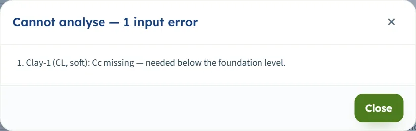
When a value cannot be used, Analyze opens a window titled Cannot analyse — 1 input error (or “N input errors”) with the numbered messages, and nothing is calculated. The bar stays Not analysed. Typing zero in a box that must be positive gives a stop:
| When | Message |
|---|---|
| Cc is zero or negative in a layer that is compressed | “Clay-1 (CL, soft): Cc missing — needed below the foundation level.” |
| e0 or Cr is negative | “Clay-1 (CL, soft): e0 missing — needed below the foundation level.” (or Cr) |
| With the mv method, mv is zero | “Clay-1 (CL, soft): mv missing — needed below the foundation level.” |
| γ is zero | “Clay-1 (CL, soft): γ is missing.” |
| γsat is zero | “Clay-1 (CL, soft): γsat is missing.” |
The compressibility is only asked where a layer is compressed, below the foundation level and above zlim; a layer above the foundation level needs only its unit weights.
Warnings
A warning does not stop the analysis. The Warnings window opens by itself after Analyze, the Results and Report tabs show a bar with the first warning and a Warnings (N) button, and the Analyze bar turns to a warning colour and shows the count. The window lists the warnings and then the assumptions of this analysis: the removed load, the excavation plan, the calculation depth, the stress path, where the settlement is measured from, and the time curve.
| When | Message |
|---|---|
| qgross is below qremoved | “The gross pressure is below the removed overburden (qnet < 0): the loading does not bring the stresses back to the initial state.” With 30 kPa the foundation settlement is 0 and the card adds that the ground ends 17.4 mm above its original level. |
| OCR below 1 | “8 slices had σ′p below σ′v0 (OCR < 1): σ′p = σ′v0 was used — under-consolidated clay is outside the scope.” |
| A laboratory σ′p below σ′v0 | “43 slices had σ′p below σ′v0 (laboratory σ′p < σ′v0): σ′p = σ′v0 was used — under-consolidated clay is outside the scope.” (the count follows your values) |
| γsat not above γw | “Clay-2 (CH, firm): γsat ≤ γw — the effective stress does not grow through this layer.” |
| The effective stress after the excavation is below 0.1 kPa | “4 slices had σ′exc below 0.1 kPa after the excavation: σ′exc = 0.1 kPa was used (the e – log σ′ law is unbounded near zero stress; the swelling of these slices is a model limit).” For example with γsat just above γw. |
| Cv missing in a compressed layer | “No time curve: Cv is missing for Clay-2 (CH, firm).” The settlement is calculated; the time columns and the Time view are empty. |
| The excavation reaches the bottom of the profile | “The excavation reaches the bottom of the soil profile (30.00 m).” With the profile rule a second one follows: “No soil between the foundation level and the calculation depth: nothing to consolidate.” and the results read 0. |
Notes on the screen
- “Results cleared — the inputs can be edited.” appears after Edit inputs.
- “The soil profile ends above zlim: Clay-3 is taken to continue …” is the note under the calculation depth when the profile is shorter than zlim; the report repeats it.
- “The soil below zlim is not compressed: the stress increase there is less than 10 % of q.” is the note when the profile is deeper.
- “Enter p between 5 % and 50 % and the size of the foundation.” shows instead of the read-outs when p or the size cannot be used.
Good practice and common mistakes
- Say where the settlement is measured from. After an excavation, Snet (206.9 mm here) and Sc from the excavation base (311.3 mm) answer different questions; the heave is reported next to them.
- Take Cs from the swelling branch of the test. Left empty, Cs = Cr is used and the report says so; a larger Cs raises the heave and the reloading together.
- Check σ′p against σ′v0. A laboratory σ′p below the initial stress is replaced by σ′v0 and warned; the slice table shows the regime of every slice.
- Decide what lies below the profile. With the influence depth the last layer is extended to zlim (here by 23.94 m); if rock or dense gravel lies there, choose Bottom of the profile.
- Keep the slices thin enough. The default 0.50 m is fine for the example; thin layers need a smaller Δz.
- Use Cv from the field when you can. The time curve follows Cv and the drainage path; a layer with a sand lens drains differently from the double-drainage assumption.
- Read the stop and the warnings. A zero in a required box stops the analysis; a warning does not, but it changes the numbers.
- Keep a record. The model is kept in this browser, but a file from Save to file… and the report travel with the project.
Frequently asked questions
What does the Consolidation settlement module calculate?
The primary consolidation settlement of clay layers under a rectangular or strip foundation, slice by slice along the stress path (swelling, reloading, recompression, virgin compression), the excavation heave, and the settlement against time by Terzaghi’s theory. For the example it gives a heave of −104.4 mm, a settlement of the foundation of +206.9 mm and t90 of 17 years.
Why is the settlement of the foundation less than the loading settlement?
The settlement is measured from the original ground by default. The excavation made the clay swell (heave −104.4 mm), and the load first recovers that heave: Snet = Sc + heave = 311.3 − 104.4 = 206.9 mm. Choose Reset to zero before loading to see 311.3 mm measured from the heaved excavation base.
What are Cs, Cr and Cc doing?
Cs governs the swelling on unloading and the reloading back to the initial stress, Cr the recompression from the initial stress to the preconsolidation pressure σ′p, and Cc the virgin compression beyond it. If Cs is empty, Cr is used.
How is the calculation depth chosen?
With the influence depth rule the settlement is summed down to where the stress increase under the centre has fallen to p (5 to 50 %, default 10) of q. For the 20 × 30 m raft that is 50.94 m below the foundation level. With Bottom of the profile it stops at the last layer.
What happens if my profile is shorter than the calculation depth?
The last layer is taken to continue down to the calculation depth with the same properties, and the drawings, the table and the report say so (“continued from 30.00 to 53.94 m (assumed)”). Choose Bottom of the profile if a stiff stratum lies below the profile.
Can I use granular layers or the immediate settlement?
No. Every layer is clay and only primary consolidation is calculated. The immediate settlement is in the two Elastic settlement modules, and Settlement 2D combines both over a profile of clay and sand layers.
What if the load is smaller than the removed overburden?
The module warns that qgross is below qremoved. The load then only brings the clay back part of the way along its swelling line: for 30 kPa the foundation settlement is 0 and the ground ends 17.4 mm above its original level.
Can I drag or move anything on the drawing?
No. The drawings are not interactive apart from the chips that show or hide parts. Every value is typed in the Model tab, and the Section view follows it. After Analyze the inputs are locked until you press Edit inputs.
Does the module remember my inputs?
Yes. Every change is kept in this browser, and the page opens on the model you last worked on, analysed or not. Save to file writes a .gtrv file, Quick Save keeps named versions in the browser, and Reset to defaults returns to the example.
Which units and signs can I use?
SI · kN, SI · tf and US, and the sign convention settlement + (default) or settlement −, all in the header and all changeable after Analyze. The drawings stay in m · kPa · mm. The Calculations tab keeps the classical sign.
How are t50 and t90 found?
Each layer follows Terzaghi’s solution with its Cv and drainage path (Hdr = H/2 for double drainage, H for single); the settlement of the profile is the sum of the layers’ degrees of consolidation times their Sc, and t50 and t90 are the times when that sum reaches 50 % and 90 % of the total.
What does the report contain?
A cover with your project details and a key-information table, then eight parts: introduction and scope, soil profile and parameters, excavation, foundation and calculation depth, stress path and assumptions, consolidation settlement, slice by slice, time-dependent consolidation and a summary, with the drawings. It saves as PDF or Word after Analyze.