

What the module calculates
Settlement 2D gives the total settlement of a foundation on a layered profile of clay and sand: the immediate (elastic) settlement of every layer plus the consolidation settlement of the cohesive layers, with the settlement–time curve. The foundation is a flexible rectangle or strip, placed at the bottom of an excavation if you enter one. The stresses, the strains and the settlement are drawn as colour bands over the section through the centre of the foundation.
- Cohesive layers (clay, silt) settle immediately, undrained, with Eu and ν = 0.5, and then consolidate along their stress path: the excavation unloads and swells them, the foundation reloads them with Cs, Cr up to σ′p and Cc beyond it (or with mv).
- Granular layers (sand, gravel) settle immediately and drained, with E′ and ν′; they do not consolidate.
- The immediate part uses Steinbrenner’s influence factors layer by layer; the stress increase uses Boussinesq. Both are summed down to the calculation depth: the depth where the stress increase under the centre has fallen to p % of q, or the bottom of the profile.
- Results: the settlement of the centre of the flexible foundation, of its corner (edge for a strip) and of a rigid foundation, the excavation heave, the settlement of every layer and every slice, and t50 and t90 of the consolidation.
Which settlement module for which job
- Only clay layers, with the full consolidation path and no elastic part: Consolidation settlement.
- The immediate settlement of clay layers alone: Elastic settlement, cohesive; of sand and gravel layers alone: Elastic settlement, granular.
- This module when the profile has both kinds of layer and you want the total, with the colour bands and the time curve.
- The stress increase alone, for other loaded shapes: the Stresses in a soil mass family.
The module gives the settlement. The bearing capacity of the foundation (see the Bearing capacity family), secondary compression, and the structural effect of differential settlement are checked with your own design checks. The family page lists the four settlement modules.
Before you start: what you need
| What | Notes |
|---|---|
| The profile From: the borehole logs | For each layer the depth of its bottom, the kind (cohesive or granular), γ and γsat. The layers run from the ground surface down without gaps. |
| The stiffness From: tests and correlations | Eu for each clay layer, E′ and ν′ for each sand or gravel layer, in MPa. |
| The consolidation data From: oedometer tests | For each clay layer e0, Cc, Cr, optionally Cs, OCR (or σ′p), Cv, and the drainage; or mv for the mv method. |
| The groundwater From: the borehole logs | The depth zw of the water table below the ground surface. |
| The excavation and the foundation From: the foundation design | The excavation depth (the foundation level), the width B and length L of the foundation (or a strip), and the gross pressure qgross at the foundation level. |
Quick start in eight steps
- Open the module and choose the units
Open Settlement 2D from the Settlement family. Pick SI · kN, SI · tf or US in the header; the Sign selector next to it chooses whether settlement is shown positive or negative.
- Enter the soil profile
In Soil profile type the bottom of each layer, its kind, name, γ and γsat; + Add layer adds a layer at the bottom.
- Enter E and ν, then the consolidation data
In Elastic parameters type E (and ν′ of the granular layers); in Compressibility type the clay data.
- Enter the water table, the excavation and the foundation
Type zw in Groundwater; choose Yes or No in Excavation and its depth; in Foundation choose the shape and type B, L and qgross.
- Choose the analysis settings
In Analysis Settings choose the compressibility method, the definition of σ′p, the calculation depth, the slice thickness and whether the time curve is wanted.
- Press Analyze
Press Analyze at the foot of the Model tab. The inputs lock and the drawing shows the Contours view.
- Read the answer
The Results tab gives Se, the consolidation settlement, the total, the heave, the corner and the rigid foundation, then every layer and every slice.
- Take the working and the report
The Calculations tab writes out one slice step by step; the Report tab saves a PDF or a Word file.
The screen: five views
The layout is the one every GeoTerva module shares (workspace guide). The drawing has five views, chosen with the buttons above it; the header carries the units and the sign convention.

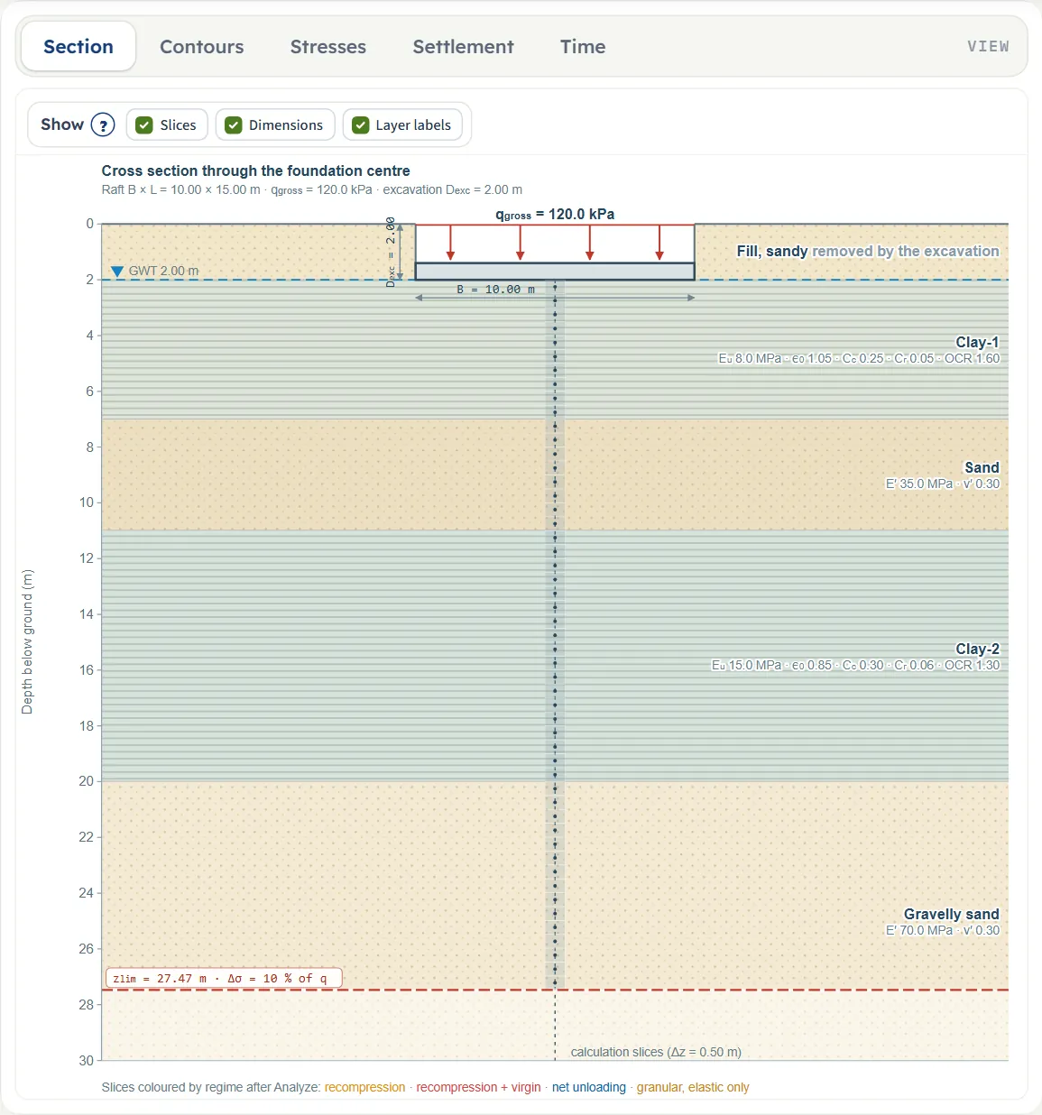
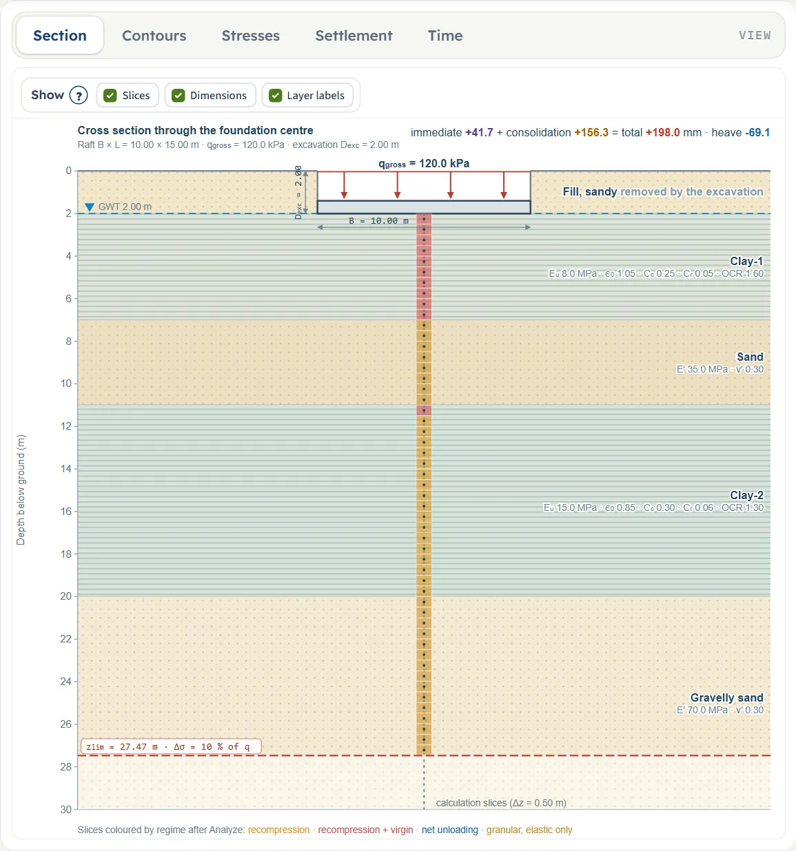
- Section is the cross section through the centre of the foundation, drawn to scale: the layers with their kind and parameters, the water table, the excavation, the foundation, the calculation slices and the calculation depth zlim. It follows the inputs as you type; after Analyze it also gives the immediate, consolidation, total and heave values at the top. Show has three chips: Slices, Dimensions and Layer labels.
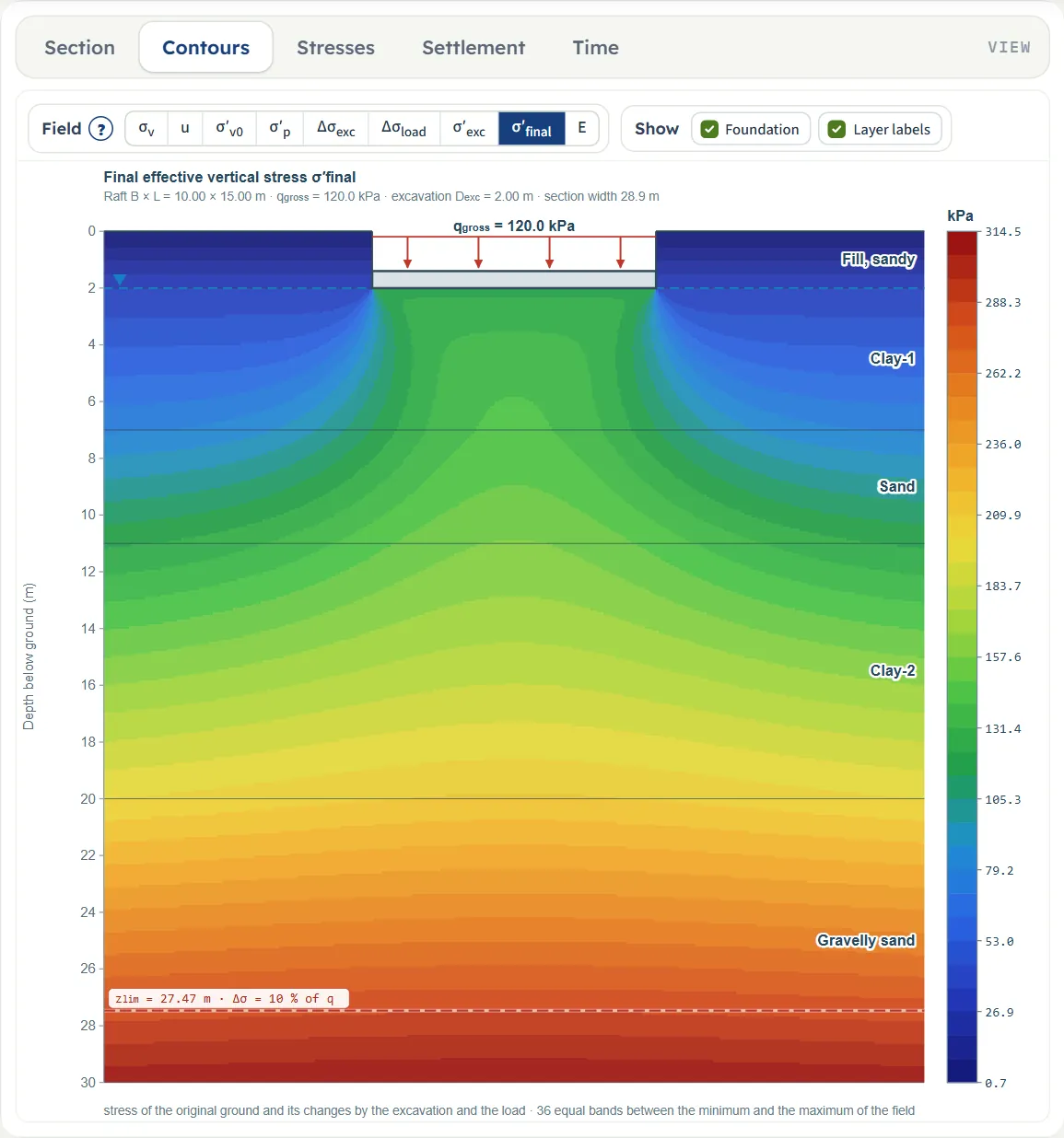
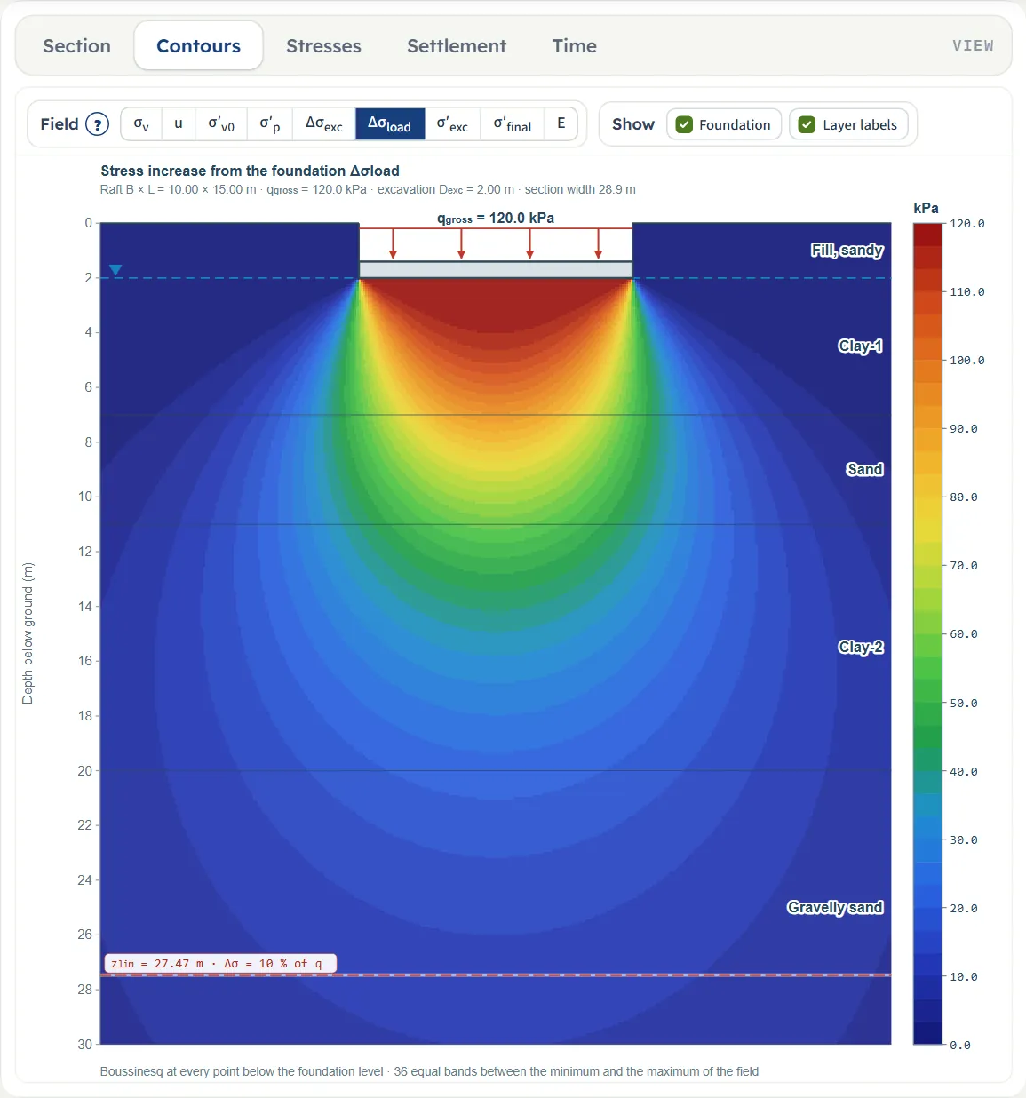
- Contours paints one field over the whole section in colour bands.
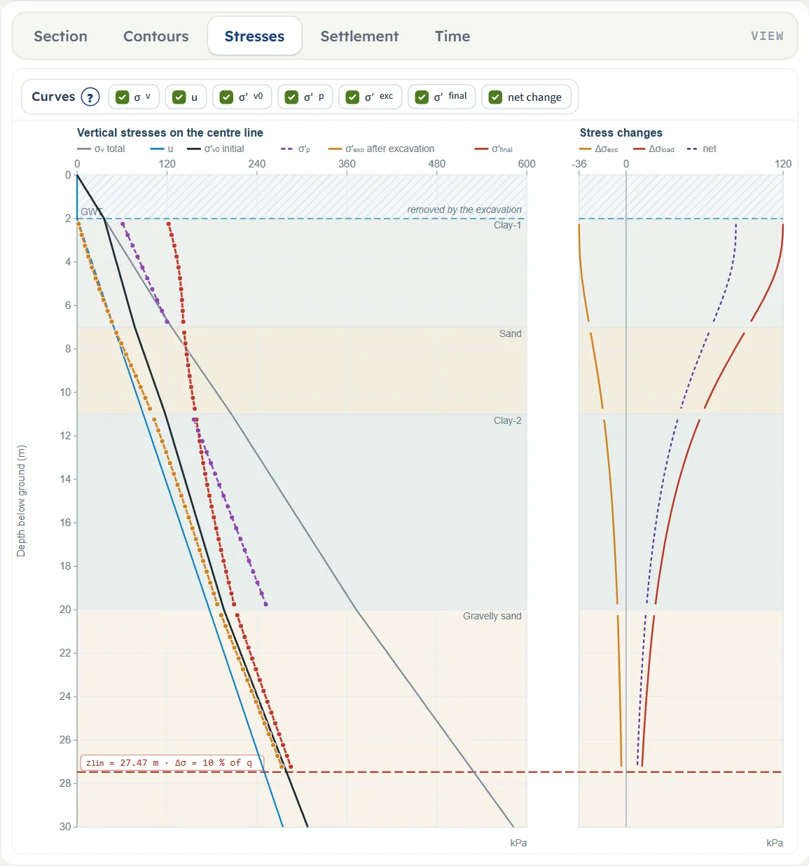
- Stresses draws the vertical stresses on the centre line against depth, with the stress changes at the right.
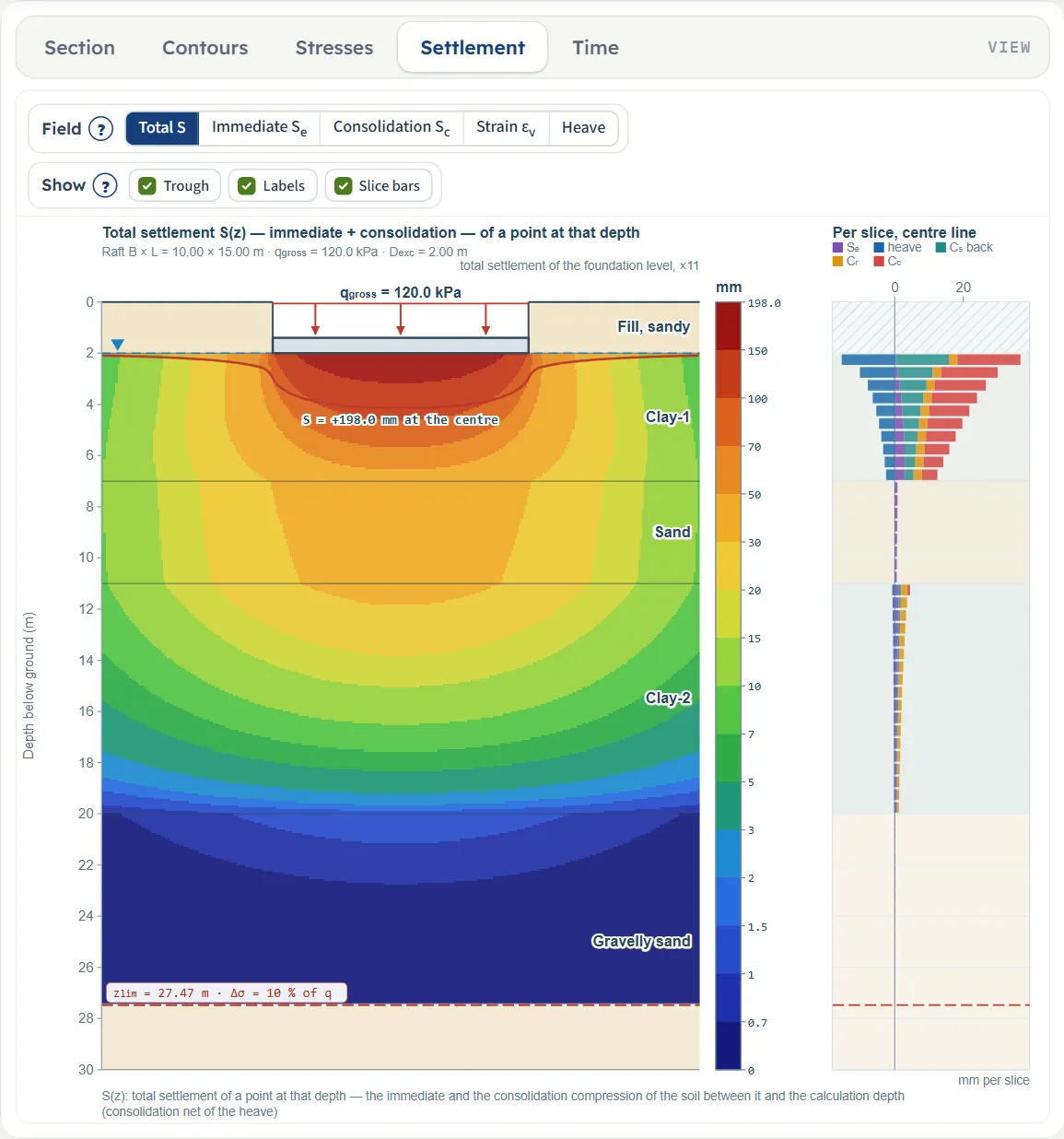
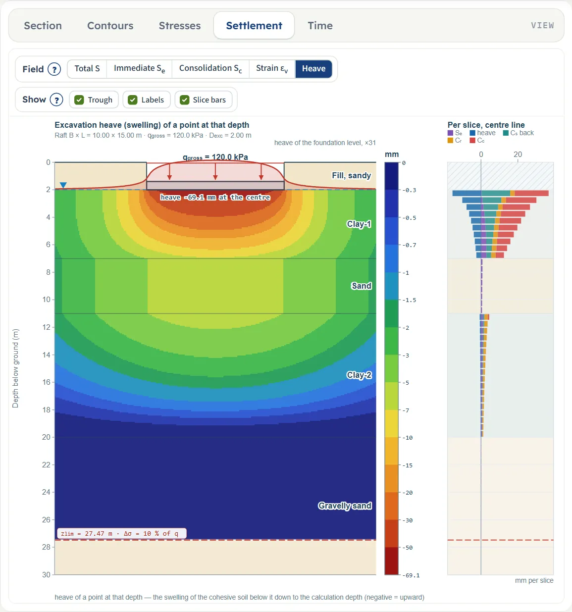
- Settlement paints the settlement, strain or heave of a point at every depth, with the compression of every slice at the right.
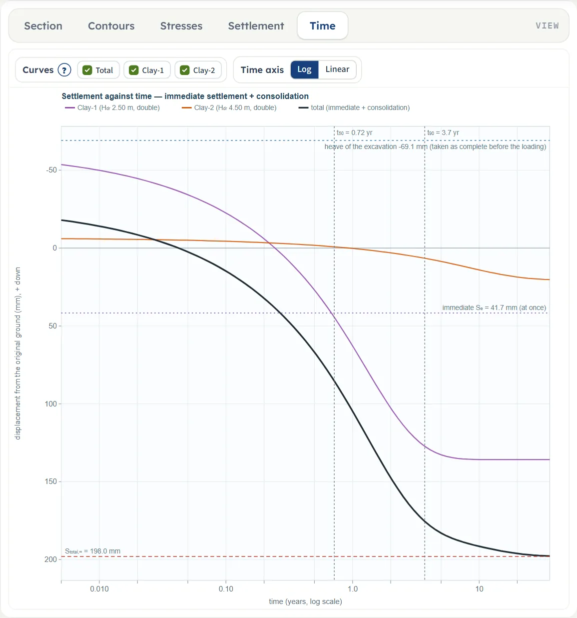
- Time draws the settlement against time.
Open the module and the drawing shows Contours, which stays empty until you press Analyze; choose Section to see the profile as you enter it. Edit inputs after an analysis returns the drawing to the Section.
Contours
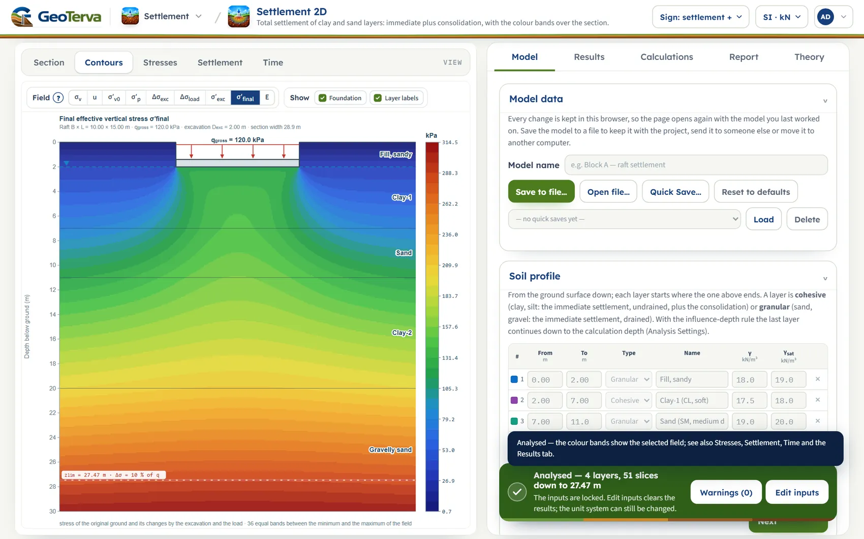
The Field buttons choose the quantity: σv, u, σ′v0, σ′p, Δσexc, Δσload, σ′exc, σ′final (the default after Analyze) and E. The legend gives the value at the boundary of the bands: 36 equal bands between the minimum and the maximum of the field. The ? beside Field explains the quantities. Show has two chips, Foundation and Layer labels.
Stresses
Curves has seven chips: σv, u, σ′v0, σ′p, σ′exc, σ′final and net change. The hatched band at the top is the part removed by the excavation.
Settlement
The Field buttons are Total S, Immediate Se, Consolidation Sc, Strain εv and Heave. The value at a point is the compression of the soil between that point and the calculation depth, so the value at the foundation level on the centre line is the settlement of the Results tab. The colours are classes (1 · 1.5 · 2 · 3 · 5 · 7 × 10 to the power n, from 1/300 of the maximum up), so that the small movements at depth keep colours of their own. Show has Trough (the exaggerated settlement of the foundation level), Labels and Slice bars (the immediate, heave, swelling-recovery, Cr and Cc parts of every slice).
Time
The curves are the total and one per cohesive layer, as the displacement from the original ground (the heave is taken as complete before the loading), with Se drawn as present at once, the final value, and t50 and t90 of the whole profile. Curves has a chip for the total and one for each cohesive layer. Time axis switches between Log and Linear. The view needs the time curve switched on and Cv in the clay layers.
What you can drag
Nothing. The drawings are pictures of the model: change the values in the Model tab and the drawing follows. There are no zoom buttons, the wheel does not zoom and the drawing cannot be panned. A table row in the Results tab opens its calculation (see Calculations).
Entering the model, section by section
The Model tab has eight sections: Model data, Soil profile, Elastic parameters, Compressibility, Groundwater, Excavation, Foundation and Analysis Settings. Click a section title to open or close it; Next and Back at its foot walk you through them. Analyze waits in a bar at the foot of the tab. Units are shown under each label; defaults are shown in SI · kN and convert when you change the units. Emptying most boxes leaves the previous value in the model, so a box cannot be left blank by accident; the exceptions are named below.
Model data
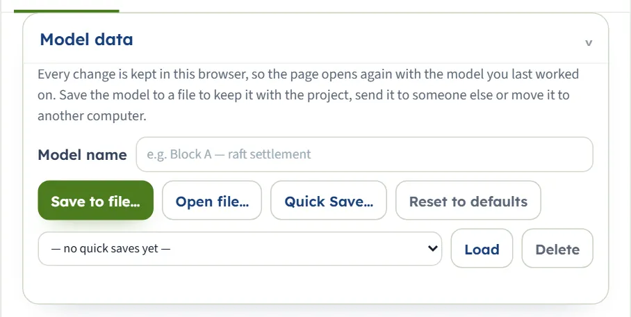
The model name, Save to file… (a .gtrv file in your downloads folder), Open file…, Quick Save… with its list, Load and Delete, and Reset to defaults. Quick Save… asks for a name; an existing name asks “Replace it?”. Delete asks for confirmation. Reset to defaults returns the example without asking and says “The inputs are back at the module defaults, and this is now the model kept in the browser.” A file that is not a model gives “Not a model file: …” in red.
Soil profile
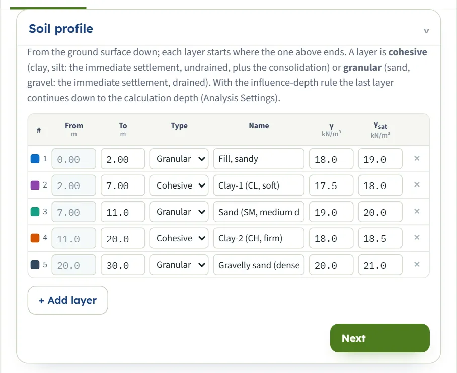
One row per layer, from the ground surface down. From is filled in (the bottom of the layer above); you type To. A To that is not below From is not accepted. Type is Cohesive or Granular. + Add layer adds a cohesive layer 2 m thick at the bottom with γ = 18.5 and γsat = 19.0 kN/m³ and clay data (Eu 15 MPa, e0 0.9, Cc 0.3, Cr 0.05, mv 0.0003 1/kPa, Cv 1 m²/yr, OCR 1.2); × deletes a layer (the last one cannot be deleted) and the layers below move up. Changing a layer to cohesive fills in the same clay data if it has none.
| Field | Default | Limits |
|---|---|---|
| To (bottom of the layer), m · ft | 2 · 7 · 11 · 20 · 30 m | Below From |
| Type | Granular · Cohesive · Granular · Cohesive · Granular | Cohesive or Granular |
| Name | Fill, sandy · Clay-1 (CL, soft) · Sand (SM, medium dense) · Clay-2 (CH, firm) · Gravelly sand (dense) | Text |
| γ, kN/m³ · t/m³ · pcf | 18.0 · 17.5 · 19.0 · 18.0 · 20.0 | Unit weight above the water table |
| γsat, kN/m³ · t/m³ · pcf | 19.0 · 18.0 · 20.0 · 18.5 · 21.0 | Below the water table |
With the influence-depth rule the last layer continues down to the calculation depth when the profile ends above it (see Analysis Settings).
Elastic parameters
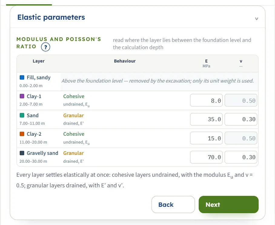
One row per layer, with the depth range of the layer. A cohesive row says “undrained, Eu” with ν = 0.50 fixed; a granular row says “drained, E′” and takes ν′. A layer entirely above the foundation level shows “Above the foundation level — removed by the excavation; only its unit weight is used.”; a layer below the calculation depth shows that it is not compressed. The ? beside Modulus and Poisson’s ratio opens a note on choosing E.
| Field | Default | Limits |
|---|---|---|
| E, MPa · kg/cm² · ksf | 8 · 35 · 15 · 70 MPa (the compressed layers) | Above 0; empty or 0 gives a stop |
| ν′ (granular only) | 0.3 | 0 to 0.49 |
Compressibility
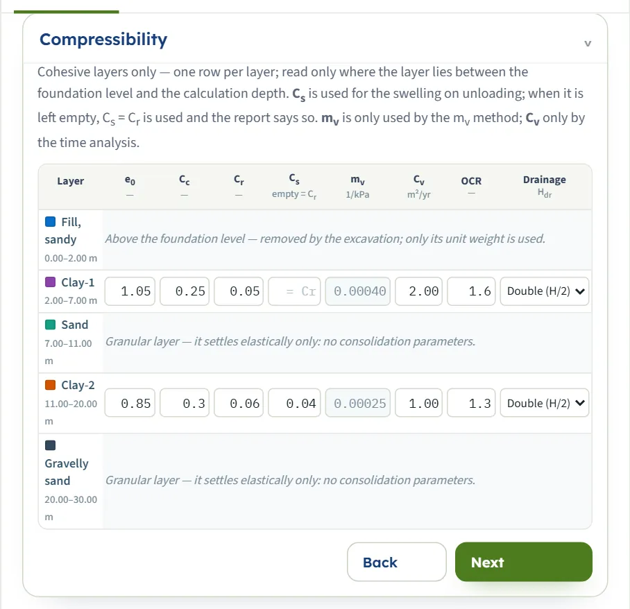
One row per cohesive layer that is compressed; the other rows say why they are not (“Granular layer — it settles elastically only: no consolidation parameters.”). The table fits the width of the panel. The boxes of the method you did not choose are greyed: mv with the e – log σ′ method, and e0, Cc, Cr, Cs with the mv method. Cv is used only when the time curve is on. The OCR column becomes σ′p when you choose the laboratory value.
| Field | Default | Limits |
|---|---|---|
| e0 | 1.05 · 0.85 | — |
| Cc · Cr | 0.25, 0.05 · 0.30, 0.06 | — |
| Cs: empty = Cr | empty · 0.04 | Emptying it is accepted |
| mv, 1/kPa | 0.00040 · 0.00025 | — |
| Cv, m²/yr | 2.00 · 1.00 | — |
| OCR, or σ′p in kPa | 1.6 · 1.3 (or 90 · 150 kPa) | OCR from 1 |
Drainage is Double (H/2) (water leaves through the top and the bottom of the layer; the default) or Single (H). H is the thickness of the layer below the foundation level, so the drainage path Hdr of the 5 m of Clay-1 below the 2 m excavation is 2.5 m. When Cs is empty the swelling uses Cr and the Warnings window says so (“Cs not given — Cs = Cr = 0.05 is used for the swelling.”). The module changes Cr and Cs together in that case: with Cs empty, Cr = 0.10 instead of 0.05 changes the heave of the default example from −69.1 to −131.6 mm.
Groundwater
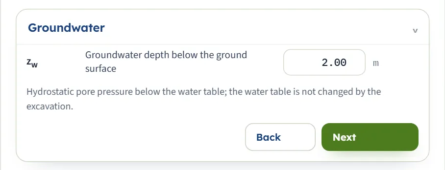
One value: the depth zw of the water table below the ground surface. Pore pressure is hydrostatic below it and the water table is not changed by the excavation. A negative value is taken as 0.
| Field | Default | Limits |
|---|---|---|
| zw, m · ft | 2.00 m | 0 or more |
Excavation
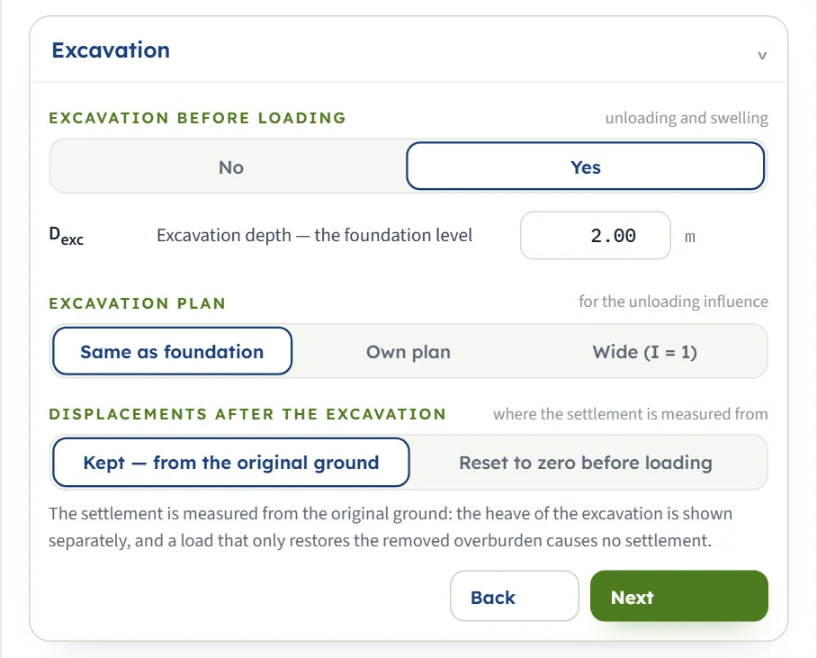
Yes or No for an excavation before loading; with Yes the excavation base is the foundation level, the removed load qremoved is the initial effective overburden there, and the clay layers swell. A depth of 0 is the same as No. Excavation plan gives the plan that unloads: Same as foundation, Own plan (type Bexc and Lexc) or Wide (I = 1) (the unloading acts fully at every depth). Displacements after the excavation chooses where the settlement is measured from: Kept — from the original ground (the heave is reported separately and the consolidation is Sc + heave) or Reset to zero before loading (the settlement is measured from the heaved base, so it includes the recompression of the heave). A note under the buttons explains the choice you made.
| Field | Default | Limits |
|---|---|---|
| Dexc, m · ft | 2.00 m | 0 or more |
| Excavation plan | Same as foundation | Three buttons |
| Displacements | Kept — from the original ground | Two buttons |
Foundation
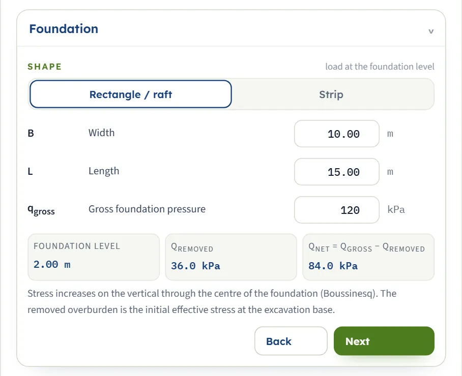
Rectangle / raft or Strip; a strip has no length. Three read-outs follow the inputs: the foundation level, qremoved and qnet = qgross − qremoved. qgross is the gross pressure at the foundation level; the immediate settlement uses qnet.
| Field | Default | Limits |
|---|---|---|
| B, m · ft | 10.00 m | At least 0.1 m |
| L, m · ft | 15.00 m | At least 0.1 m |
| qgross, kPa · t/m² · ksf | 120 kPa | 0 or more |
Analysis Settings
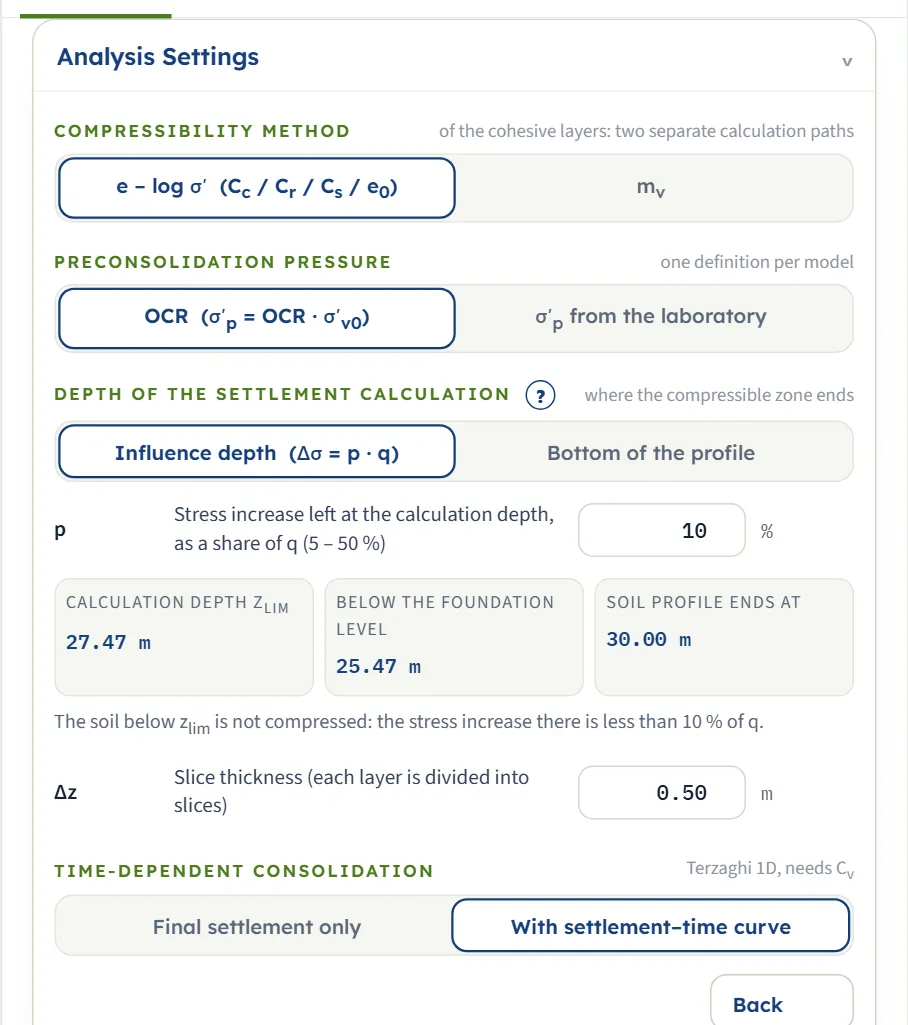
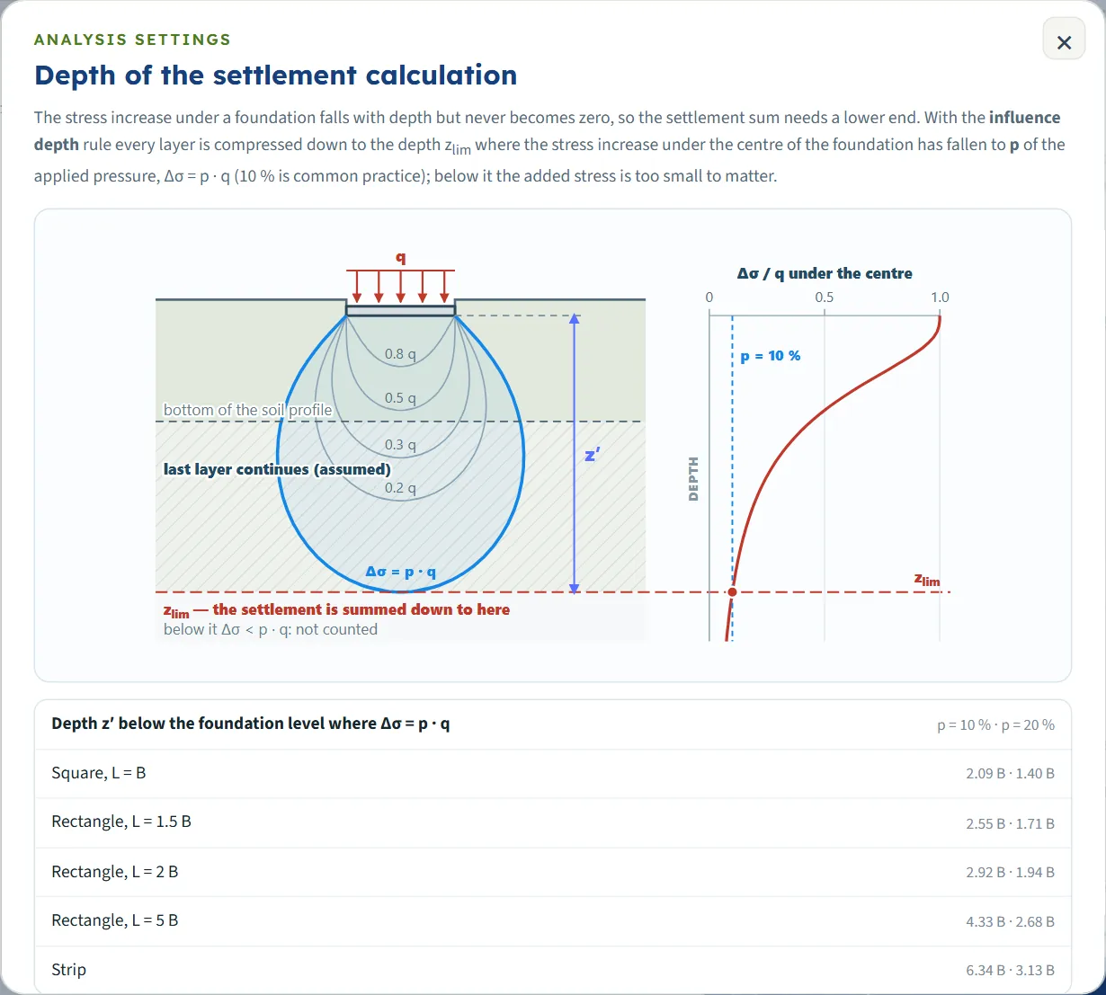
Compressibility method: e – log σ′ (with Cc, Cr, Cs, e0) or mv, a separate linear path. Preconsolidation pressure: OCR (σ′p = OCR · σ′v0) or σ′p from the laboratory. Depth of the settlement calculation: Influence depth (Δσ = p · q) or Bottom of the profile; with the first, type p (5 to 50 %; typed values outside are brought to the limit). Three read-outs give zlim, the depth below the foundation level and the end of the profile, and a note says whether the profile is continued or cut. The ? beside the heading opens a note with a drawing and the depth z′ for common shapes. Slice thickness Δz (0.05 to 2 m) is the largest thickness of a slice. Time-dependent consolidation: Final settlement only or With settlement–time curve.
| Field | Default | Limits |
|---|---|---|
| Method · σ′p definition | e – log σ′ · OCR | Two buttons each |
| Calculation depth · p | Influence depth · 10 % | 5 to 50 % |
| Δz, m · ft | 0.50 m | 0.05 to 2 m |
| Time curve | With settlement–time curve | Two buttons |
Slices are made in each layer between the foundation level and zlim, split at the water table, each at most Δz thick. In the default example the water table coincides with the top of Clay-1, so the cohesive layer is cut into 10 slices of 0.50 m and the profile into 51 slices in all. A thinner slice changes the answer very little: Δz = 0.25 m gives 198.1 mm, 2 m gives 197.0 mm.
Choosing the method and the options
Calculation depth
The influence-depth rule sums down to where the stress increase under the centre has fallen to p of q; the default is 10 %. When the profile ends above that depth the last layer is taken to continue with the same properties (the Results table says “continued from 30.00 to 65.40 m (assumed)”, for example for a strip of 10 m); when the profile is deeper the soil below is not compressed. Bottom of the profile stops at the end of the last layer, which suits a stiff stratum right below it: the default example then sums to 30.00 m and gives 198.3 mm against 198.0 mm. A larger p stops earlier (20 %: 194.7 mm; 5 %: 199.0 mm).
Displacements kept or reset
With Kept — from the original ground a load that only restores the removed overburden causes no settlement; with Reset to zero before loading the same load settles by as much as the base had heaved. Use reset when the excavation stays open long enough for the heave to develop before the structure is built. In the default example kept gives S = 198.0 mm and reset gives 267.1 mm; both measures are always shown in the Results table.
Excavation plan
The unloading follows the plan you name. For the default example Same as foundation gives a total of 198.0 mm, Own plan of 20 × 30 m gives 184.5 mm and Wide (I = 1) gives 174.7 mm; the heave grows from −69.1 to −80.4 and −89.6 mm because more of the unloading reaches the clay.
The mv method
With mv the same mv serves the unloading and the reloading; the default example gives 254.8 mm in total (heave −91.3 mm). The method does not use e0, Cc, Cr, Cs or σ′p.
σ′p from the laboratory
With σ′p from the laboratory the module takes the σ′p you type for each clay layer, never below σ′v0. The default values 90 and 150 kPa are below the stress of the deeper slices, so the analysis gives a warning and a total of 248.8 mm; type the values of your tests.
Analyze and read the results
Press Analyze. The bar counts through six steps (initial stresses, excavation unloading, foundation loading, immediate settlement, consolidation, time), then reads “Analysed — 4 layers, 51 slices down to 27.47 m” and shows Warnings (0) and Edit inputs. A toast says “Analysed — the colour bands show the selected field; see also Stresses, Settlement, Time and the Results tab.” The module stays on the Model tab and the drawing changes to Contours; open Results for the numbers. The inputs are locked until you press Edit inputs (“Results cleared — the inputs can be edited.”); the units and the sign can still be changed.
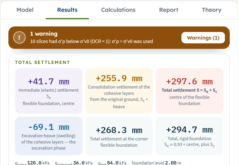
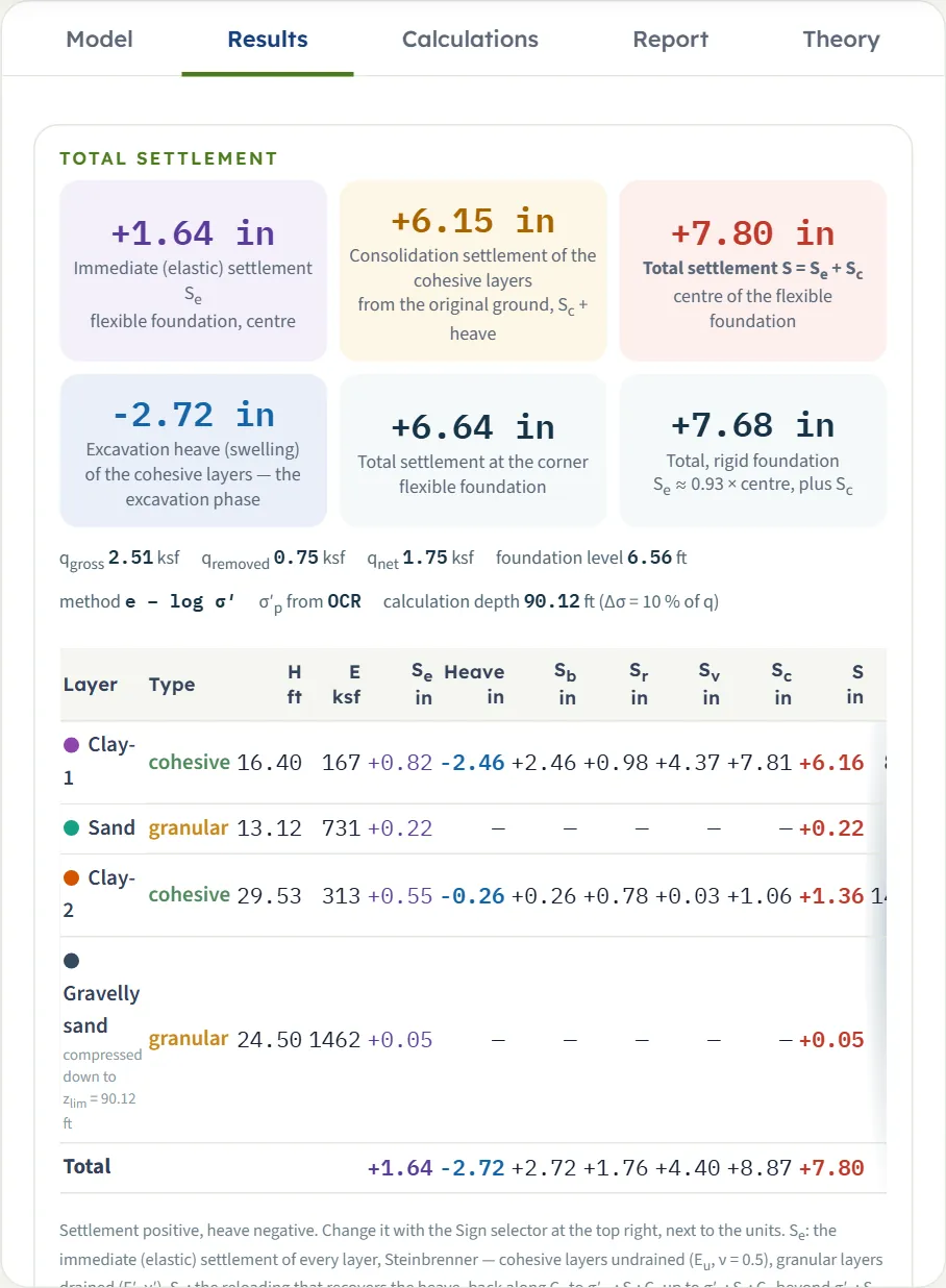
The Total settlement block has six cards. Their values for the default example:
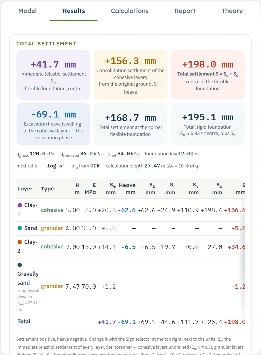
| Card | Value |
|---|---|
| Immediate (elastic) settlement Se, flexible foundation, centre | +41.7 mm |
| Consolidation settlement of the cohesive layers (from the original ground, Sc + heave) | +156.3 mm |
| Total settlement S = Se + Sc, centre of the flexible foundation | +198.0 mm |
| Excavation heave (swelling) | −69.1 mm |
| Total settlement at the corner of the flexible foundation (the edge, for a strip) | +168.7 mm |
| Total, rigid foundation: Se ≈ 0.93 × centre, plus Sc | +195.1 mm |
A line under the cards repeats qgross, qremoved, qnet, the foundation level, the method, the source of σ′p and the calculation depth. The signs follow the Sign selector: settlement positive and heave negative, or the reverse (the vertical displacement positive upward), in the cards, the tables, the drawings and the report; the Calculations tab keeps the classical signs and says so.
The table of the layers
One row per layer that is compressed, with H (the thickness compressed), E, Se, the heave, Sb (the reloading that recovers the heave, back along Cs), Sr (Cr up to σ′p), Sv (Cc beyond it), Sc = Sb + Sr + Sv, the layer total S, and with the time curve Hdr, t50 and t90. The table is wider than the panel at some sizes: scroll it sideways to reach the last columns. The layer total is Se + (Sc + heave) when the displacements are kept, Se + Sc when they are reset.
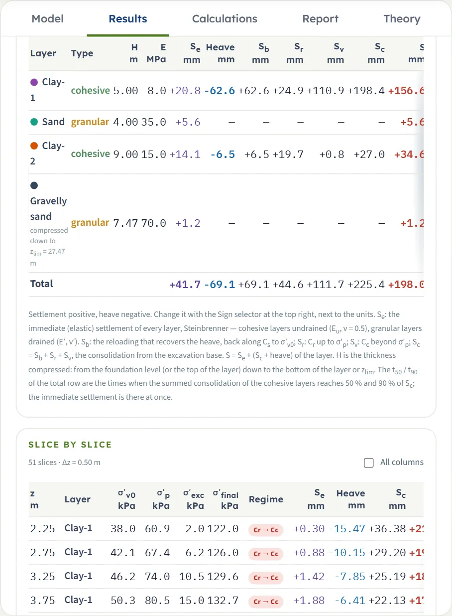
| Layer | Se · heave · Sc | S · t50 · t90 |
|---|---|---|
| Clay-1 H 5.00 m, E 8.0 MPa | +20.8 · −62.6 · +198.4 | +156.6 mm · 0.62 · 2.7 yr |
| Sand H 4.00 m, E 35.0 MPa | +5.6 · — · — | +5.6 mm |
| Clay-2 H 9.00 m, E 15.0 MPa | +14.1 · −6.5 · +27.0 | +34.6 mm · 4.0 · 17 yr |
| Gravelly sand H 7.47 m (to zlim) | +1.2 · — · — | +1.2 mm |
| Total | +41.7 · −69.1 · +225.4 | +198.0 mm · 0.72 · 3.7 yr |
Each layer total is in millimetres; the Sc of Clay-1 (+198.4) is larger than its net contribution (+135.8) because the heave of −62.6 mm is recovered first. The Total row gives t50 and t90 of the whole profile: the times when the summed consolidation of the cohesive layers reaches 50 % and 90 % of Sc; the immediate settlement is there at once.
Slice by slice
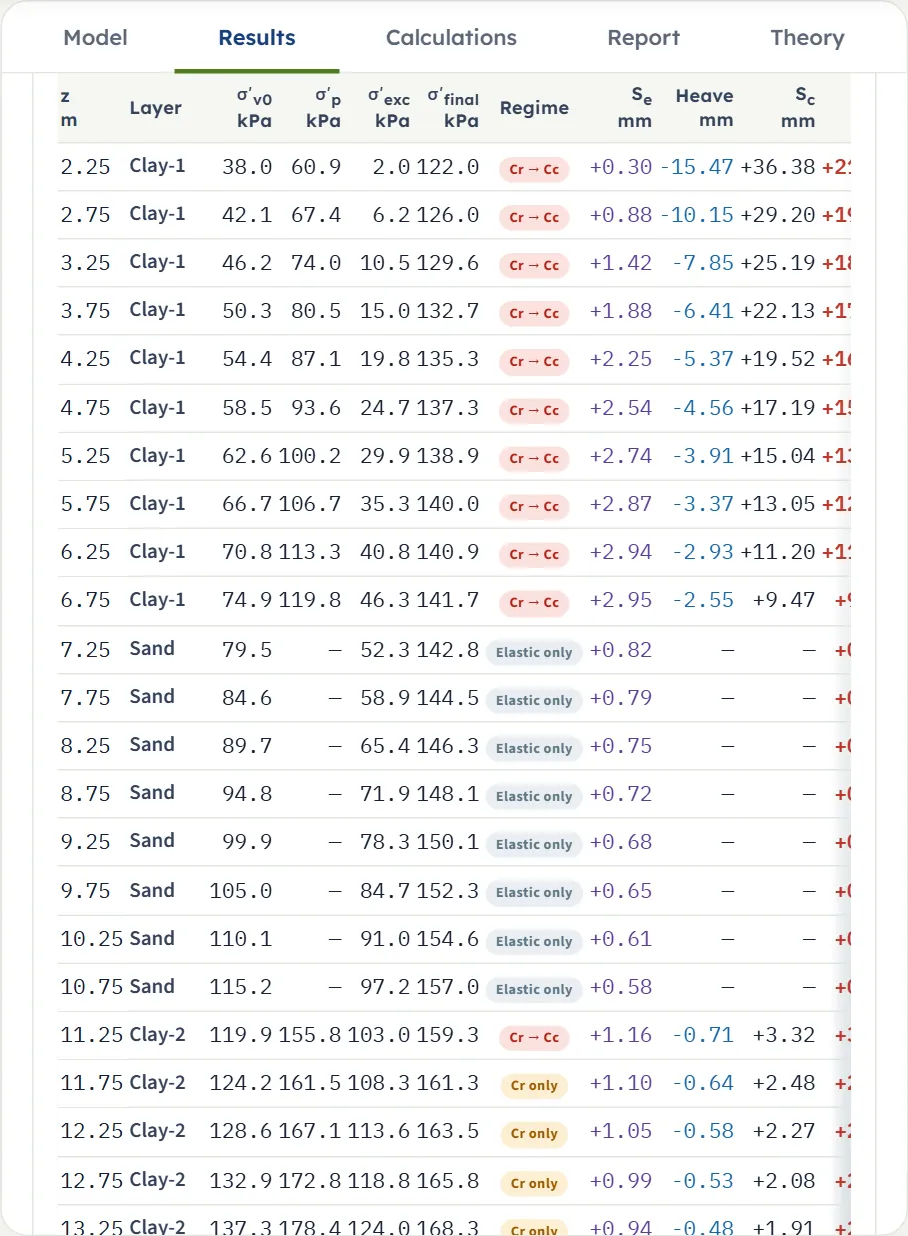
Below the layers a table lists every slice: z, the layer, σ′v0, σ′p, σ′exc, σ′final, the Regime and Se, heave, Sc and S. All columns adds E, ΔH, σv0, u0, Δσexc, Δσload, Sb, Sr and Sv. The regime says which index carries the loading: Cr → Cc (recompression then virgin), Cr only, Cc only, Cs (heave recovered), Cs (net unloading), mv, or Elastic only for a granular slice. A click on a row opens its calculation.
Warnings
When the analysis finds something to say, the Warnings window opens by itself after Analyze; it lists the warnings and the assumptions of the analysis. A coloured bar at the top of the Results and Report tabs repeats the first warning with a Warnings button, and Warnings (n) in the bar of the Model tab opens the window again.
Calculations tab, Report and Theory
Calculations
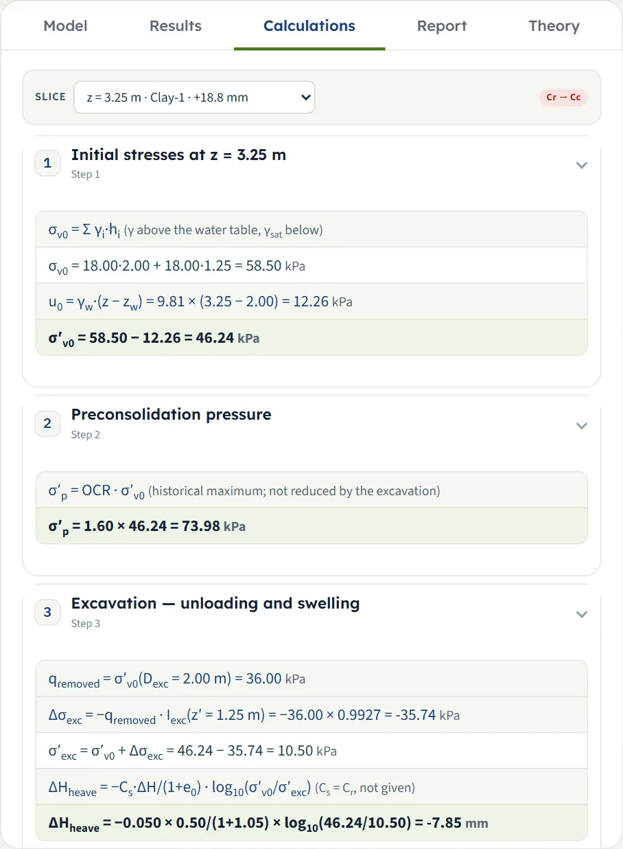
The tab writes out one slice with your numbers; choose the slice in the Slice list (z, layer and the slice settlement), or click a row of the slice table. The regime of the slice shows at the right. The steps are numbered and open with a click: 1 initial stresses, 2 preconsolidation pressure (clay), 3 excavation — unloading and swelling (clay), 4 foundation loading — Boussinesq, 5 immediate (elastic) settlement of the slice, 6 consolidation compression of the slice (clay), 7 slice, layer and total, and 8 time (for a clay layer with the time curve on). Granular slices have no steps 2, 3, 6 and 8.
Report
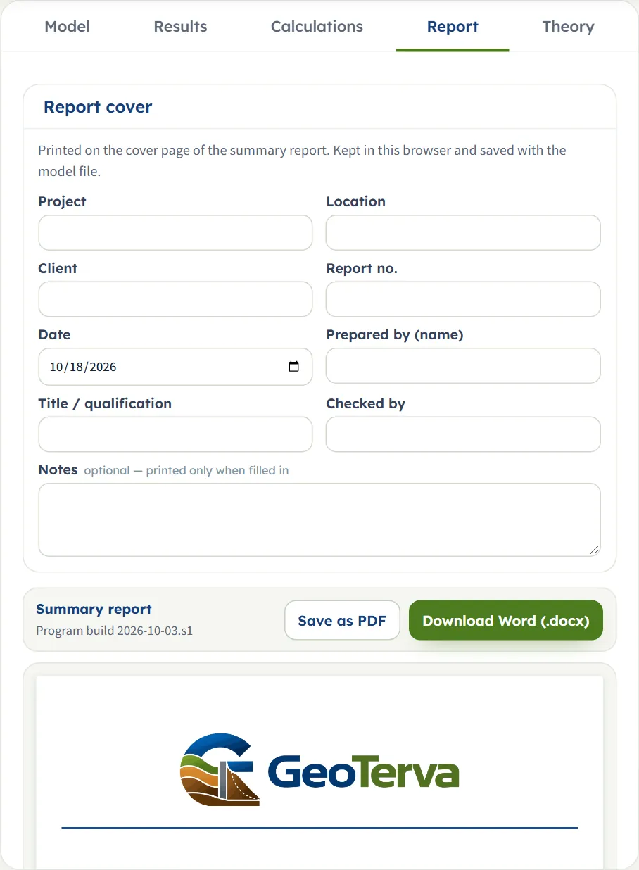
The Report tab has a cover form (Project, Location, Client, Report no., Date, Prepared by (name), Title / qualification, Checked by, Notes), kept in the browser and saved with the model file, and a live preview of the summary report with Save as PDF (opens a print window: choose “Save as PDF”) and Download Word (.docx). The buttons work after Analyze. The report has eleven parts: introduction and scope; soil profile and parameters; excavation, foundation and calculation depth; method and assumptions; immediate settlement; consolidation settlement; total settlement; slice by slice; time-dependent consolidation (when the time curve is on); summary; references. It carries the drawings of the Section, Stresses, Contours, Settlement and Time views.
Theory
The Theory tab has 21 sections: scope; cohesive and granular layers; immediate settlement; Steinbrenner’s influence factors; the layered profile and the net pressure; the stress path of the cohesive layers; slices and initial stresses; preconsolidation pressure; excavation; the stress increase; the depth of the calculation; compression regimes; where the settlement is measured from; the mv method; flexible and rigid foundations; total settlement; time-dependent consolidation; the colour-band fields; sign convention and assumptions; outside the scope; references.
Worked example
The default example: a raft of 10 × 15 m, qgross = 120 kPa, at the bottom of a 2 m excavation; water table at 2 m; Clay-1 from 2 to 7 m (Eu 8 MPa, e0 1.05, Cc 0.25, Cr 0.05, OCR 1.6, Cv 2 m²/yr), sand from 7 to 11 m (E′ 35 MPa), Clay-2 from 11 to 20 m (Eu 15 MPa, e0 0.85, Cc 0.30, Cr 0.06, Cs 0.04, OCR 1.3, Cv 1 m²/yr), gravelly sand from 20 to 30 m (E′ 70 MPa); fill of 18 kN/m³ above. Influence depth with p = 10 %, Δz = 0.5 m, displacements kept.
The removed load and the calculation depth
- qremoved = σ′v0(2.00 m) = 18.0 × 2.00 = 36.0 kPa; qnet = 120.0 − 36.0 = 84.0 kPa.
- The depth below the foundation level where the stress increase under the centre falls to 10 % of q is z′ = 25.47 m, so zlim = 2.00 + 25.47 = 27.47 m, above the end of the profile (30 m): Gravelly sand is compressed over 7.47 m only.
One slice by hand: 3.25 m, Clay-1
- σv0 = 18.0 × 2.00 + 18.0 × 1.25 = 58.50 kPa, u0 = 9.81 × 1.25 = 12.26 kPa, σ′v0 = 46.24 kPa; σ′p = 1.60 × 46.24 = 73.98 kPa.
- Unloading: z′ = 3.25 − 2.00 = 1.25 m, Iexc = 0.9927, Δσexc = −36.00 × 0.9927 = −35.74 kPa, σ′exc = 10.50 kPa. Heave = −0.05 × 0.50/(1 + 1.05) × log(46.24/10.50) = −7.85 mm.
- Loading: Iz = 0.9927, Δσload = 119.1 kPa, σ′final = 10.50 + 119.1 = 129.6 kPa, above σ′p: regime Cr → Cc.
- Sb = +7.85 mm (back along Cs to σ′v0), Sr = 0.05 × 0.50/2.05 × log(73.98/46.24) = +2.49 mm, Sv = 0.25 × 0.50/2.05 × log(129.6/73.98) = +14.85 mm; Sc = +25.19 mm; net of the heave +17.34 mm.
- Immediate: Se = 84.0 × (1 − 0.5²)/8000 × [F(1.50 m) − F(1.00 m)] = +1.42 mm (Steinbrenner’s F of the centre of the raft). S of the slice = 1.42 + 17.34 = 18.76 mm.
These are the numbers of the Calculations tab for that slice (σ′v0 46.24, σ′p 73.98, σ′exc 10.50, heave −7.85, Sc 25.19, S 18.76 mm), and an independent re-computation of the whole profile, written from the same formulas, gives the totals of the Results tab: Se = 41.7, Sc + heave = 156.3, S = 198.0, corner 168.7, rigid 195.1 mm, t50 = 0.72 and t90 = 3.7 years.
Time by hand
Clay-1 has 5.00 m below the foundation level, double drainage, so Hdr = 2.50 m: t50 = 0.197 × 2.50²/2.00 = 0.62 yr and t90 = 0.848 × 2.50²/2.00 = 2.7 yr. Clay-2: Hdr = 4.50 m, t50 = 0.197 × 4.50²/1.00 = 4.0 yr, t90 = 17 yr. The whole profile (0.72 and 3.7 yr) is the sum of the two curves, weighted by their Sc.
The same model in the other unit systems
Switch the units after Analyze and the cards, tables and working convert; the drawings stay in SI. US: Se +1.64 in, consolidation +6.15 in, total +7.80 in (198.0 mm / 25.4), heave −2.72 in, corner +6.64 in, rigid +7.68 in; zlim = 90.12 ft and qremoved = 0.75 ksf. SI · tf: the settlements are the same in mm; qgross = 12.2, qremoved = 3.7 and qnet = 8.6 t/m², and E is shown in kg/cm² (8 MPa reads 82).
How each input changes the answer
Each row changes one thing in the default example (total S 198.0 mm, Se 41.7 mm), run on the module. Everything else is as in the worked example.
| Change | Se, mm | S, mm |
|---|---|---|
| Default | 41.7 | 198.0 |
| qgross 60 kPa qnet = 24 kPa | 11.9 | 36.7 |
| qgross 180 kPa | 71.5 | 350.5 |
| B 5 m (L 15 m) zlim falls to 19.53 m | 33.1 | 158.1 |
| Raft 20 × 30 m zlim rises to 52.94 m | 55.2 | 266.5 |
| Strip of 10 m zlim 65.40 m, profile continued | 47.6 | 219.2 |
| No excavation foundation at the surface | 76.2 | 272.5 |
| Displacements reset | 41.7 | 267.1 |
| Water table 5 m | 41.7 | 155.8 |
| Water table 0.5 m | 48.3 | 288.0 |
| Clay-1 OCR 1.0 normally consolidated | 41.7 | 297.6 |
| Clay-1 OCR 3.0 | 41.7 | 110.7 |
| Clay-1 Cc 0.40 | 41.7 | 264.6 |
| Clay-1 e0 1.5 | 41.7 | 173.6 |
| Clay-1 Eu 16 MPa | 31.3 | 187.6 |
| Sand E′ 70 MPa | 38.9 | 195.2 |
| mv method | 41.7 | 254.8 |
The immediate settlement follows the stiffness and the net pressure but not the consolidation data; the consolidation follows the clay data, the water table, the excavation and the load. Between the first rows, S rises from 36.7 to 198.0 to 350.5 mm as qgross goes from 60 to 120 to 180 kPa, a more than proportional increase because the clay passes from recompression to virgin compression. The input with the largest effect is not the same for every model: here OCR of Clay-1 (110.7 to 297.6 mm over the range tried) and the water table (155.8 to 288.0 mm) move the answer more than the sand modulus (195.2 to 198.0 mm).
Time
| Change | t50, yr | t90, yr |
|---|---|---|
| Default (Clay-1 Cv 2 m²/yr, double drainage) | 0.72 | 3.7 |
| Clay-1 Cv 4 m²/yr | 0.37 | 2.1 |
| Clay-1 single drainage | 2.6 | 11 |
| Excavation 8 m (Clay-2 only) | 4.0 | 17 |
Cv and the drainage change only the time, not the final settlement (198.0 mm in each case).
Messages
Cannot analyse
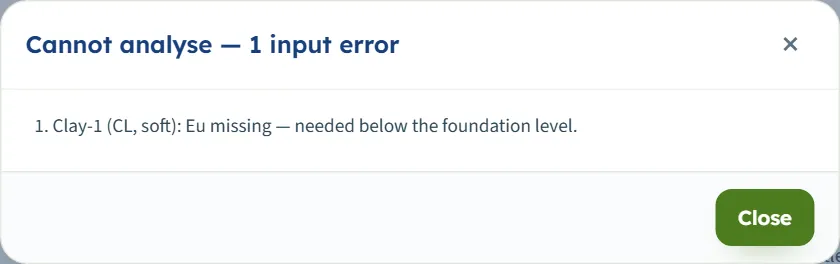
The window “Cannot analyse — 1 input error” (or 2 and more) lists what is missing; nothing is calculated and the Model tab stays editable. The ones you can reach from the screen:
- “Clay-1 (CL, soft): Eu missing — needed below the foundation level.” (the box of E was emptied; the same for E′ of a granular layer, and for the compressibility values the module says which are missing).
- “Sand (SM, medium dense): ν′ must be at least 0 and below 0.5 for a granular layer.” (the box of ν′ was emptied).
Warnings
The analysis runs and the Warnings window opens. Each is quoted as the module writes it:
- “10 slices had σ′p below σ′v0 (OCR < 1): σ′p = σ′v0 was used — under-consolidated clay is outside the scope.” (an OCR below 1; with the laboratory value the text reads “(laboratory σ′p < σ′v0)”).
- “No time curve: Cv is missing for Clay-1 (CL, soft).” (Cv is 0 with the time curve on; the settlements are still given).
- “Clay-2 (CH, firm): γsat ≤ γw — the effective stress does not grow through this layer.”
- “The net pressure is not positive (qnet = -6.0 kPa): the foundation does not load the soil beyond the removed overburden, so the immediate settlement is not positive (a negative value is an elastic rebound).” followed by “The gross pressure is below the removed overburden (qnet < 0): the loading does not bring the stresses back to the initial state.”
- “1 slice had σ′exc below 0.1 kPa after the excavation: σ′exc = 0.1 kPa was used (the e – log σ′ law is unbounded near zero stress; the swelling of these slices is a model limit).”
- “The excavation reaches the bottom of the soil profile (30.00 m).”
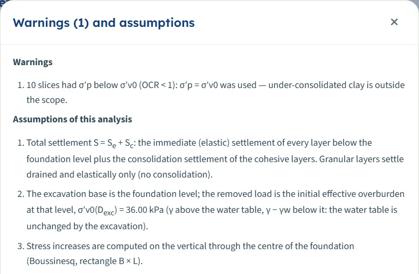
The assumptions list always follows: the sum S = Se + Sc, the removed load, the calculation depth, the continuation or cutting of the profile, the displacements, the source of σ′p and a note when Cs is empty. A model with no clay below the foundation level says “Total settlement S = Se”.
Good practice
- Check the calculation depth. The influence depth of a large raft or a strip can lie far below the last borehole layer; the profile is then continued with the properties of the last layer. Choose Bottom of the profile when a stiff stratum lies right below it.
- Split thick layers where the stiffness or the OCR changes with depth: the module takes one set of values per layer.
- Take Eu and E′ from tests or correlations suited to your soil. The immediate settlement is inversely proportional to E; the help beside Modulus and Poisson’s ratio gives the usual ranges.
- Decide the reference of the settlement (kept or reset) from how long the excavation stays open, and quote the one you used.
- Use the colour bands to look for odd results: a band that jumps at a layer boundary is the stiffness or the compressibility changing; the stress and settlement bands should die out smoothly with depth.
- Mind the unit of E: MPa in SI, ksf in US.
- Save the model to a file with the project; the quick saves live in this browser only.
Frequently asked questions
What is the difference between the immediate and the consolidation settlement?
The immediate settlement is the elastic deformation as the load is applied: for clay undrained (Eu and ν = 0.5), for sand drained (E′ and ν′). The consolidation settlement is the slow compression of the clay as the pore water leaves. Sand has only the first. The total is S = Se + Sc.
Why does the module ask for an excavation?
The foundation level is the base of the excavation. The excavation removes the effective overburden, so the clay swells; the load first recovers that heave. Choose No for a foundation at the ground surface: the default example then settles 272.5 mm instead of 198.0 mm.
What do “kept” and “reset” mean?
Kept measures the settlement from the original ground: the heave is shown on its own and a load that only restores the removed overburden causes no settlement. Reset measures from the heaved base, so the recompression of the heave counts as settlement. The default example gives 198.0 mm kept and 267.1 mm reset.
Where does the calculation depth come from?
With the influence-depth rule it is the depth where the stress increase under the centre of the foundation falls to p % of q (10 % by default), measured below the foundation level and added to its depth. The Analysis Settings read-outs show it before you analyse.
Why is the corner settlement smaller than the centre?
The foundation is perfectly flexible: its immediate settlement is largest at the centre and smallest at the corner (the edge of a strip). The consolidation is that of the centre line, so the corner total is the corner immediate settlement plus the consolidation of the centre.
What is the rigid foundation value?
A rigid foundation settles uniformly. The module takes the immediate part as 0.93 times the flexible centre value and adds the consolidation of the centre: 195.1 mm for the default example.
The heave is negative. Is that an error?
No. The classical convention shows settlement positive and heave negative. The Sign selector in the header switches to settlement negative and heave positive everywhere except the Calculations tab.
Can I leave Cs empty?
Yes. The swelling then uses Cr and the Warnings window says so. Note that changing Cr then changes the heave too.
Do my inputs survive a reload?
Yes. The page reopens on the last model, analysed if it was analysed. Reset to defaults clears it. Save to file or Quick Save keep versions.
Can I drag or zoom the drawings?
No. The drawings follow the values you type; the views and their chips are the controls.
Why is there no time curve?
The curve needs the time option on, a cohesive layer below the foundation level and Cv above 0 in every clay layer. Otherwise the Time view is empty and, for a missing Cv, a warning names the layer.
What does “continued from 30.00 to 65.40 m (assumed)” mean?
The profile ends above the calculation depth, so the last layer is taken to continue with the same properties. Choose Bottom of the profile if a stiff stratum lies below it.