

What the module calculates
Elastic settlement — cohesive gives the immediate settlement of a flexible foundation on a profile of clay and silt layers that deform undrained, right after the load is applied, at constant volume. The soil is treated as an elastic body: each layer has an undrained modulus Eu and a Poisson’s ratio of ν = 0.5, and the vertical strain is added up layer by layer, slice by slice, with the influence factors of Steinbrenner.
qnet is the pressure that the foundation adds at its own level, α and B′ select the centre or the corner of the foundation, and Is is the shape factor of Steinbrenner, which depends on the length-to-width ratio and on the depth. The settlement is summed from the foundation level down to the calculation depth zlim.
What you can describe
- A layered profile of cohesive layers, from the ground surface down, with a name, unit weights and an undrained modulus Eu for each layer.
- A rectangular (raft) or strip foundation with its width, length and gross pressure, with or without an excavation before loading.
- Groundwater at a depth below the ground, which sets the effective overburden removed by the excavation.
- The depth of the calculation: the influence depth, where the stress increase has fallen to a share p of the pressure, or the bottom of the profile (a rigid base below it).
The module gives the settlement at the centre and at the corner (the edge of a strip) of the flexible foundation and for a rigid foundation, the share of every layer, every slice with its stress and strain, the working for any slice, and a PDF or Word report. The stresses, the strain and the settlement are drawn as colour bands over the section.
Which module for what
- Clay settles twice: at once, undrained (this module), and later, as the water leaves, by consolidation. For the consolidation of the clay layers and the settlement–time curve use Consolidation settlement.
- For sand and gravel layers, which settle drained as the load is applied, use Elastic settlement — granular.
- For one profile that has both kinds of layer, with the immediate and the consolidation settlement added, use Settlement 2D.
- If you only need the stress increase under a foundation, the Stresses in a soil mass modules give it at any point. The bearing capacity of the same foundation belongs to the Bearing capacity family.
Before you start: what you need
Have these ready from your investigation and design:
| What | Notes |
|---|---|
| The soil profile | Layer depths from the ground surface, a unit weight γ above the water table and γsat below it for every layer. Every layer is cohesive: the module has no type to choose. |
| The undrained modulus Eu of each layer | In MPa (or the unit of the system you choose). The settlement is inversely proportional to Eu, so this is the number to think about most. Split a thick layer into several when the stiffness grows with depth. Enter it for the layers below the foundation level. |
| The groundwater depth zw | Below the ground surface. It matters through the effective overburden that the excavation removes. |
| The foundation | Width B, length L (or a strip), and the gross pressure qgross at the foundation level. |
| The excavation | Whether the ground is excavated before the foundation is loaded, and how deep. The foundation level is the base of the excavation. |
| The depth rule | The influence depth with a share p (10 % is the starting value), or the bottom of the profile when a rigid stratum lies right below it. |
Quick start in seven steps
- Open the module and choose the units
Open Elastic settlement — cohesive from the Settlement family. In the header pick SI · kN, SI · tf or US, and the sign convention of the displacements (Sign: settlement + is the starting choice). You can change both at any time.
- Describe the soil profile
In Soil profile give the depth of the bottom of each layer, its name and its unit weights. Press + Add layer for more layers and × to delete one.
- Give the elastic parameters
In Elastic parameters type the undrained modulus Eu of each layer. ν is fixed at 0.50.
- Set the water table and the excavation
Enter the groundwater depth in Groundwater. In Excavation choose Yes and the depth, or No.
- Describe the foundation
In Foundation choose Rectangle / raft or Strip and enter the width, the length (rectangle only) and the gross pressure. The net pressure is shown below.
- Choose how deep to calculate
In Analysis Settings keep Influence depth (Δσ = p · q) with p = 10 %, or choose Bottom of the profile.
- Press Analyze
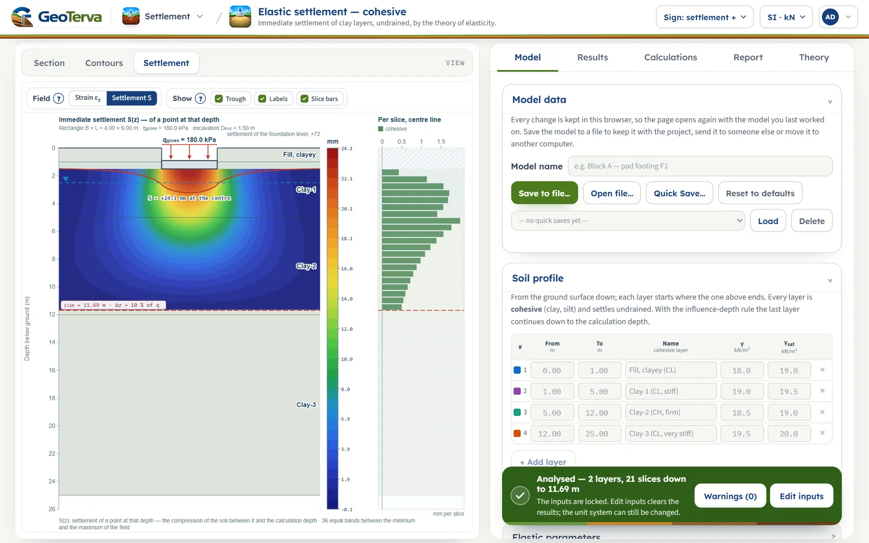
Press Analyze at the foot of the Model tab. The inputs lock and the drawing shows the settlement of the section. The numbers are on the Results tab; Calculations and Report follow.
The screen: three views of the section
The layout is the one every GeoTerva module shares, described in the workspace guide. This module has three views of the section through the centre of the foundation, chosen above the drawing, and five tabs on the right: Model, Results, Calculations, Report and Theory.
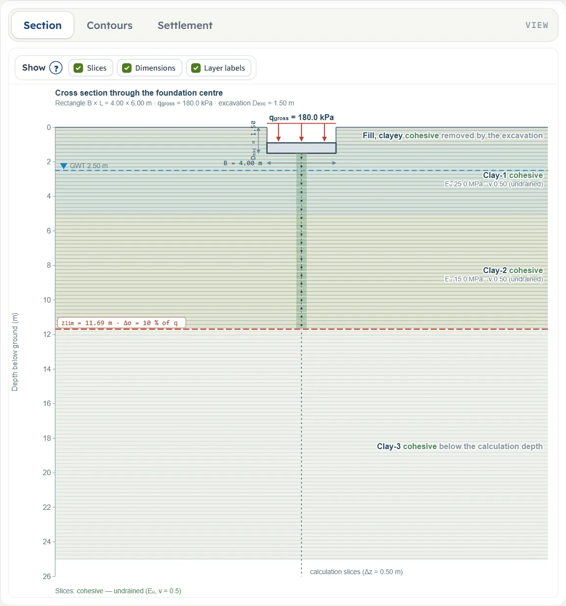
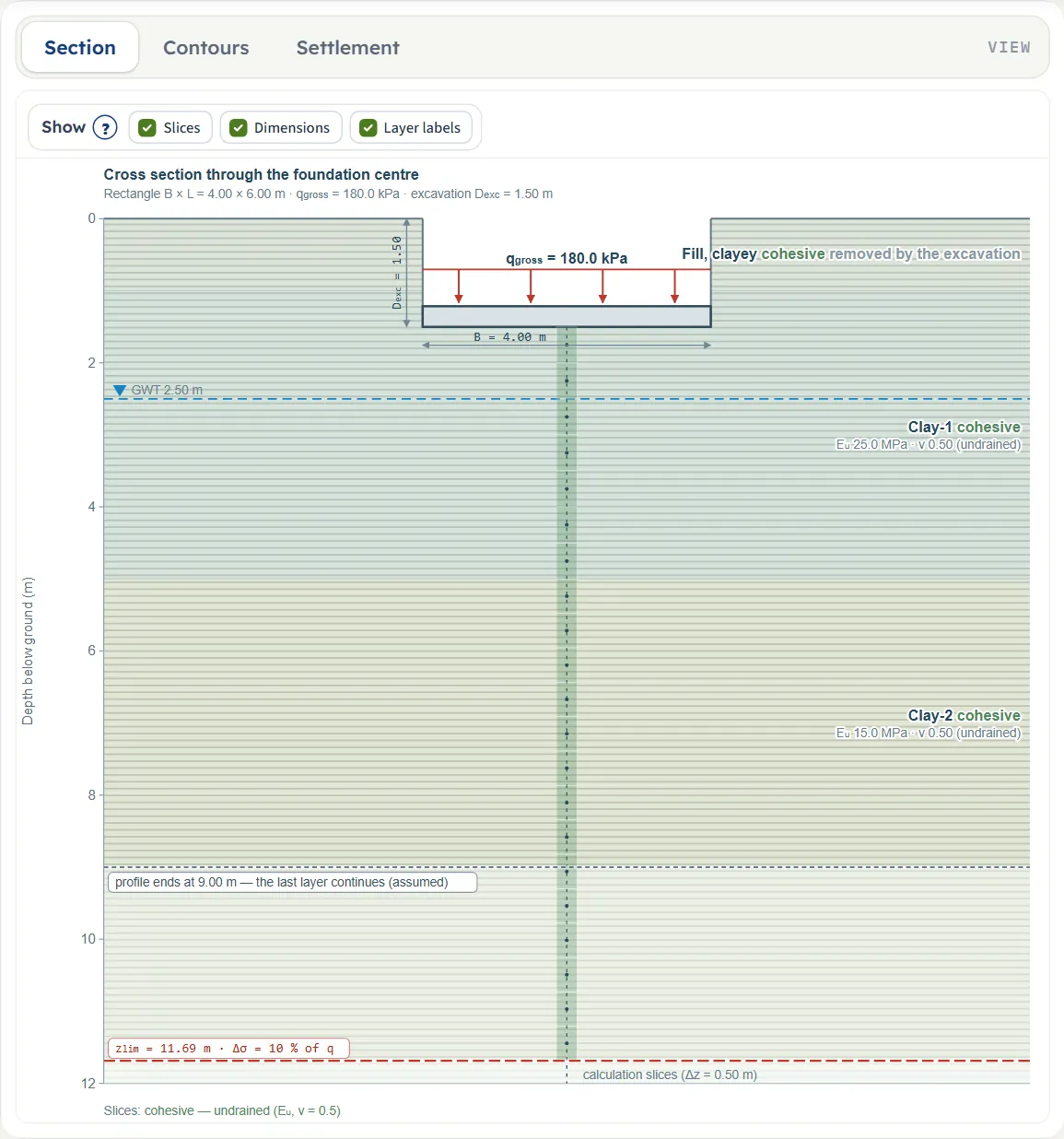
- Section is the soil profile: the layers with their names, the water table, the excavation, the foundation with its pressure, the depth scale, the calculation slices and the calculation depth zlim. It follows your inputs as you type.
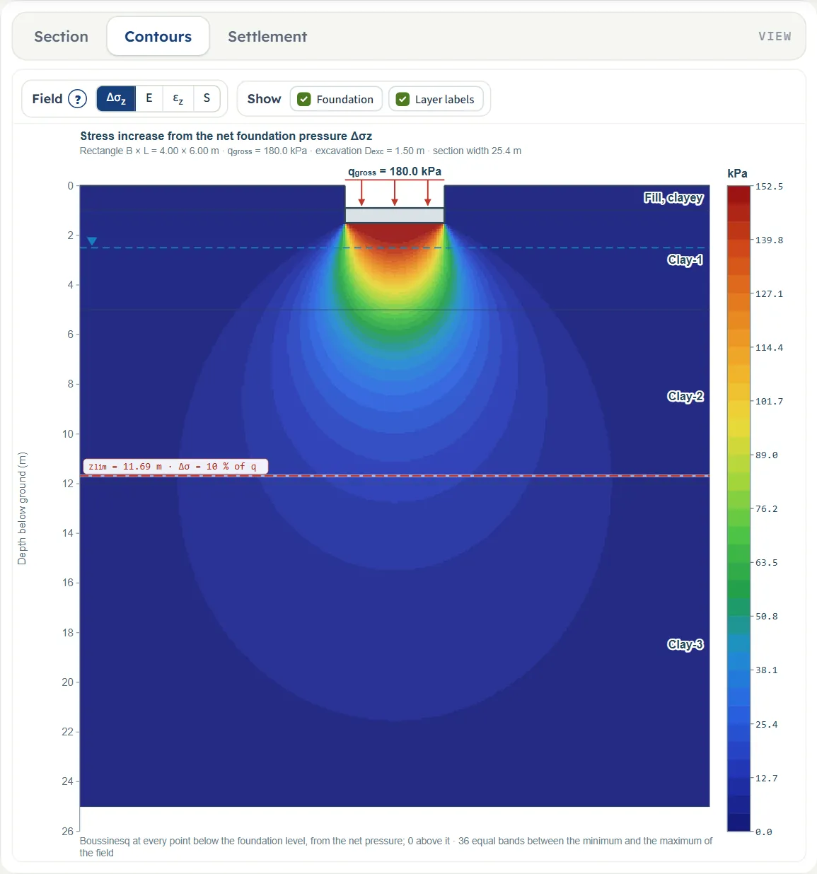
- Contours paints one quantity over the section as colour bands, with a legend: Δσz (the stress increase from the net pressure), E (the modulus of the layers), εz (the vertical strain) or S (the settlement of a point at that depth, that is, the compression of the soil between it and the calculation depth).
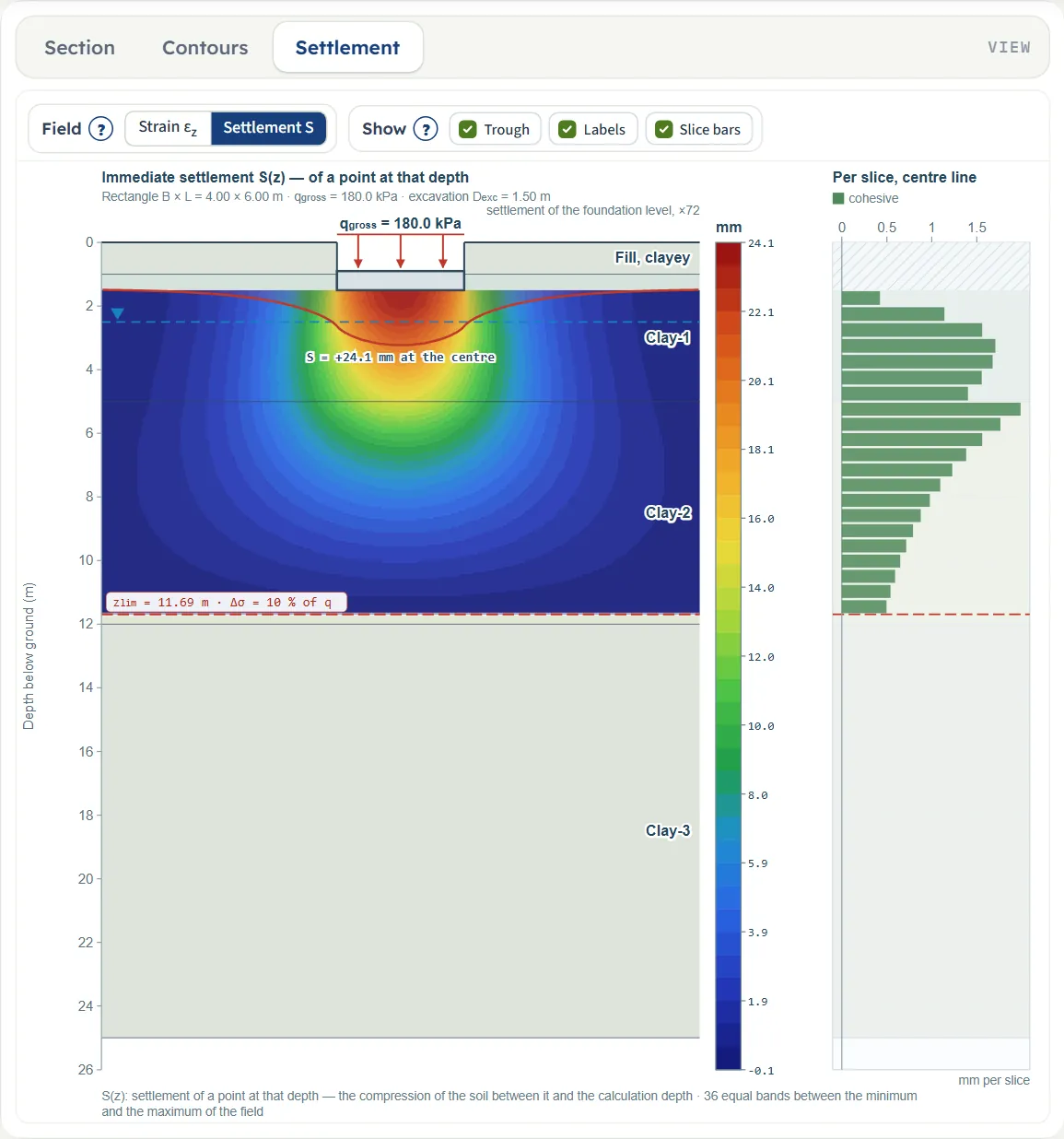
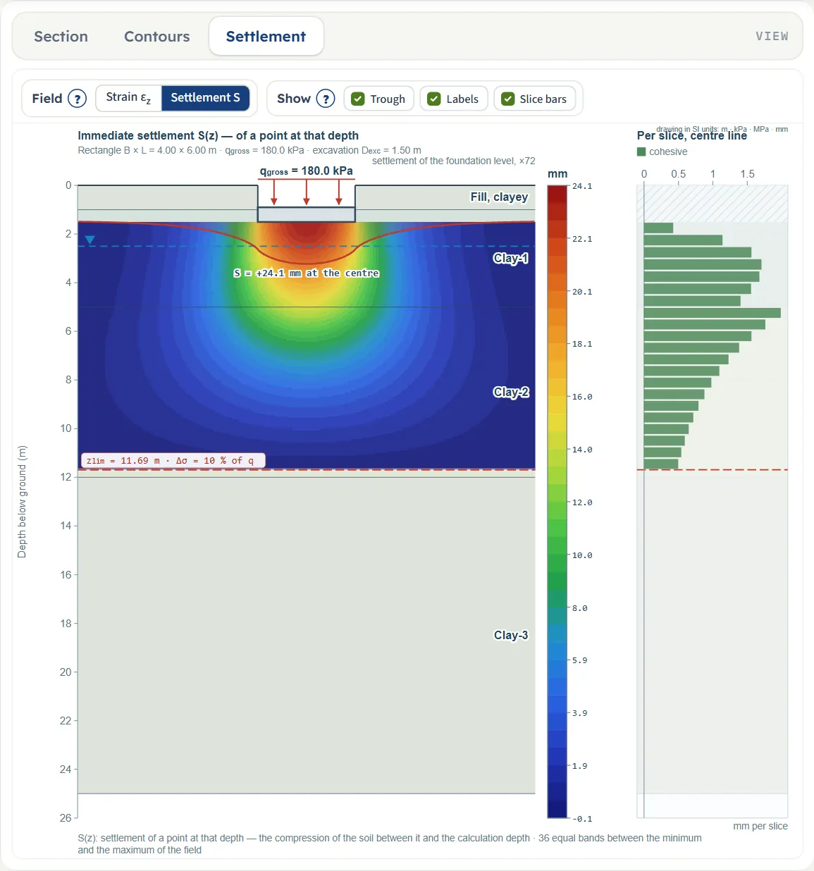
- Settlement shows Settlement S or Strain εz as colour bands, the exaggerated settlement trough of the foundation level, and a bar for every slice on the centre line. After Analyze the module opens on this view.
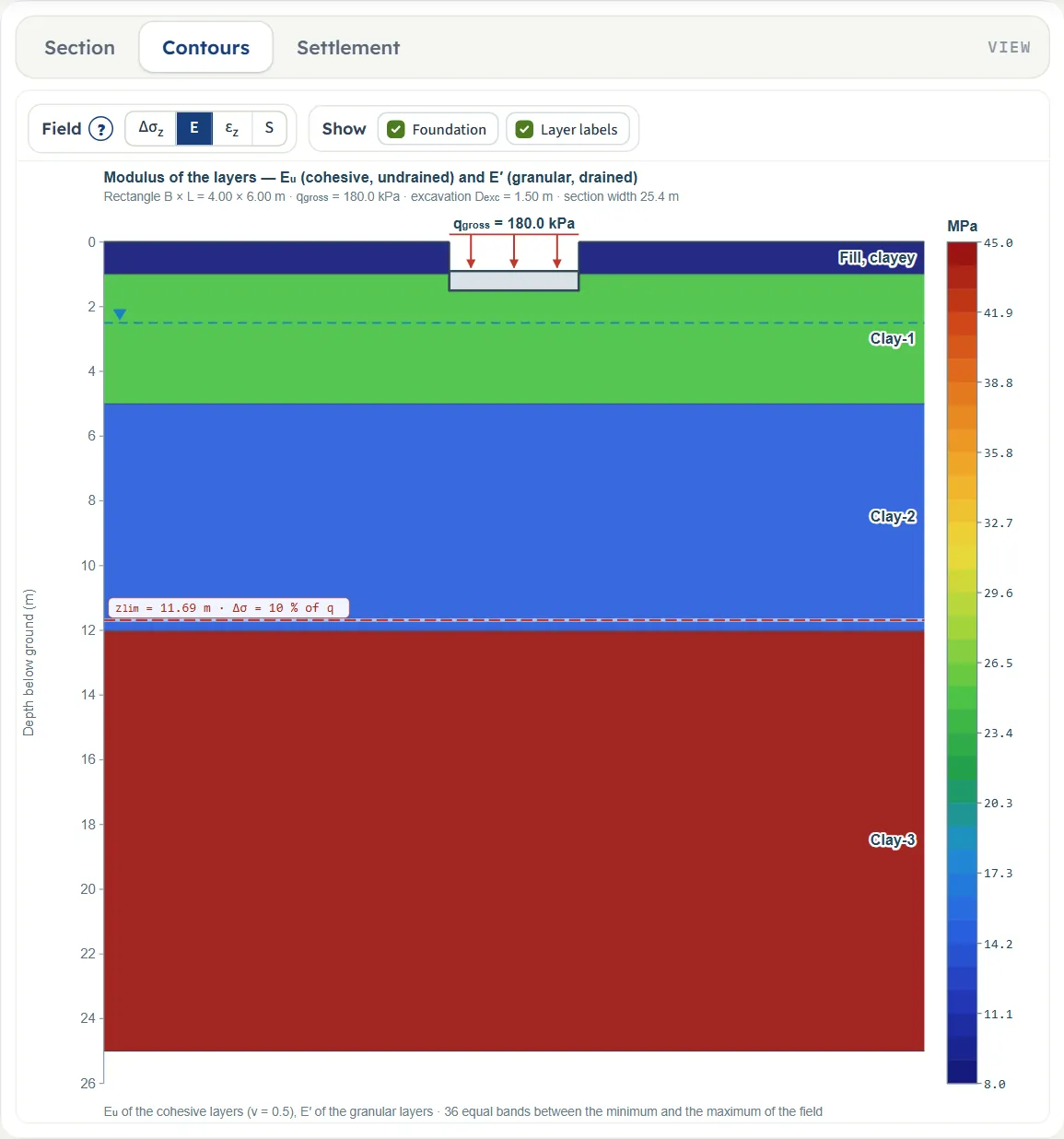
The Show chips
Each view has a Show bar of chips that switch parts of the drawing on and off. They change the drawing only, never the calculation, and they can be used before and after Analyze.
- Section: Slices, Dimensions, Layer labels.
- Contours: Foundation and Layer labels, and the Field buttons Δσz, E, εz, S.
- Settlement: Trough, Labels and Slice bars, and the Field buttons Strain εz and Settlement S.



Entering the model, section by section
The Model tab has seven sections. Model data stands on its own and can stay open; the other six are walked through one at a time: opening one closes the previous, and Next and Back at the foot of each move on. Analyze waits below the last section. Boxes show the unit of the system you chose (m · ft, kPa · ksf, and so on); the model itself is kept in SI. When you change the unit system a box may show more digits than before, because it shows the stored value converted.
Model data
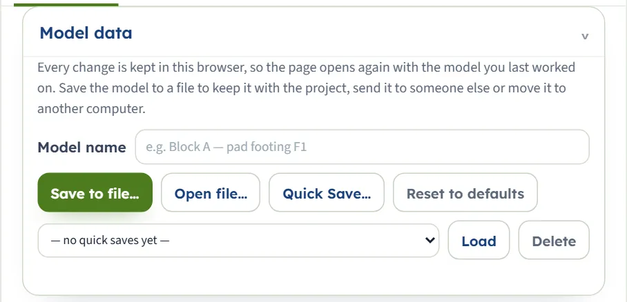
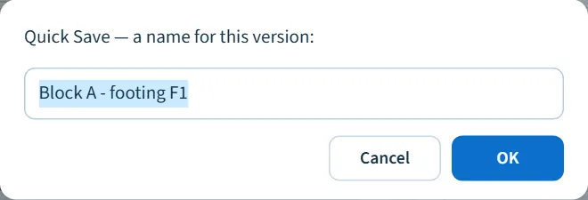
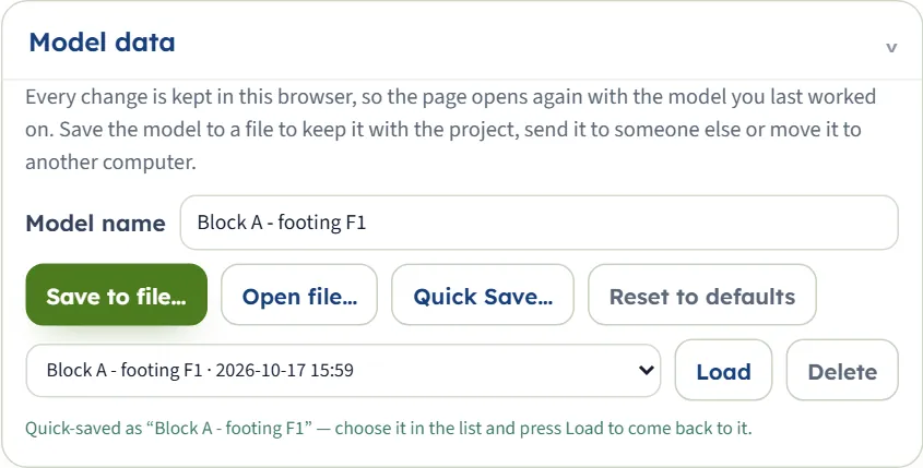
Save the model, open another, or start again. Model name is a label for the model. Save to file… writes a .gtrv file (a file window opens, or the file goes to your downloads folder). Open file… reads one. Quick Save… asks for a name and keeps this version in the list under it in this browser; choose it and press Load, or Delete it. Reset to defaults returns to the example.
Every change you make is kept in this browser automatically, so the page opens on the model you last worked on, with the results if it was analysed: a line under the buttons says so. The units and the sign convention are remembered too.
Soil profile
One row per layer, from the ground surface down: From (read-only, the bottom of the layer above, 0 for the first), To (the depth of the bottom of the layer), Name, the unit weight γ above the water table and the saturated unit weight γsat below it. Changing To moves the From of the next layer, so the profile cannot have a gap or an overlap. A To that is not below its From is ignored and the box returns to its value.
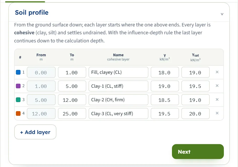
| Field (unit) | Starting values |
|---|---|
| To (m · ft) | 1.00 · 5.00 · 12.00 · 25.00 |
| Name | Fill, clayey (CL) · Clay-1 (CL, stiff) · Clay-2 (CH, firm) · Clay-3 (CL, very stiff) |
| γ (kN/m³) | 18.0 · 19.0 · 18.5 · 19.5 |
| γsat (kN/m³) | 19.0 · 19.5 · 19.0 · 20.0 |
- + Add layer adds a layer below the last one, 2 m thick, named “Layer” and its number, with γ = 19.0 and γsat = 20.0 kN/m³ and Eu = 25 MPa. Change what you need.
- × deletes a layer and the layers below move up; the last remaining layer cannot be deleted.
- With the influence-depth rule the last layer continues down to the calculation depth when the profile is shorter than that (see Analysis Settings below).
Elastic parameters
The undrained modulus E of every layer that is compressed, in MPa in SI · kN (the unit of the chosen system otherwise), and the Poisson’s ratio ν, fixed and read-only at 0.50. A layer that lies above the foundation level has no boxes: the table says it is removed by the excavation and only its unit weight is used. A layer below the calculation depth says it is not compressed. In the example the fill has no boxes for the first reason and Clay-3 for the second. The ? beside the title opens a help window on the choice of E and ν.
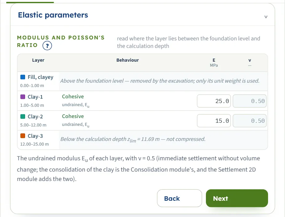
| Field (unit) | Starting values |
|---|---|
| E (MPa) | Clay-1 25.0 · Clay-2 15.0 (the fill and Clay-3 take no value in the example; their moduli are 8 and 45 MPa in the stored model) |
| ν | 0.50 for every layer |
Groundwater
One number, zw, the depth of the water table below the ground surface. The module uses it for the effective overburden removed by the excavation; the excavation does not change the water table. A negative depth is taken as 0 (the table at the surface), and an empty box keeps the previous value.
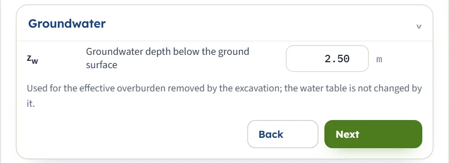
| Field (unit) | Starting value |
|---|---|
| zw (m · ft) | 2.50 |
Excavation
No or Yes. With Yes you give the depth Dexc of the excavation, which is also the foundation level: the foundation load acts at its base, and the soil above is removed (a layer that ends above it takes no part; one that it cuts is used from the foundation level down). The excavation takes off the effective overburden at its base, so the net pressure is smaller than the gross pressure. With No the pressure acts at the ground surface.
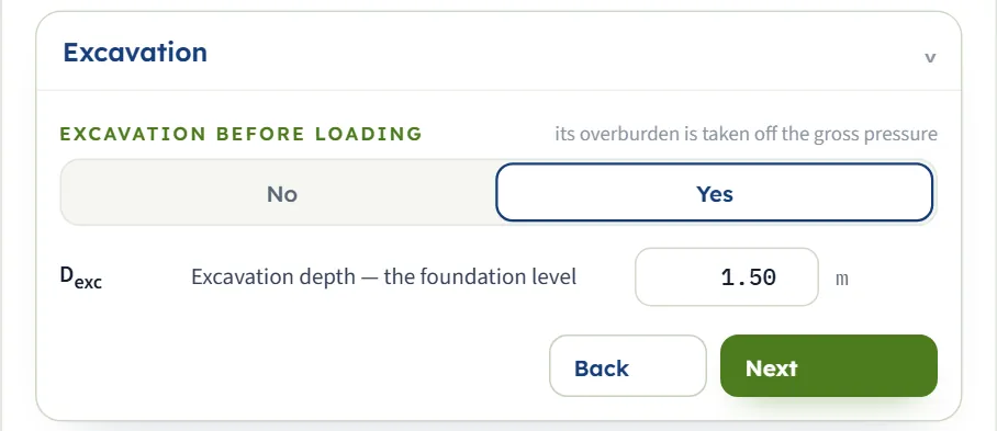
| Field (unit) | Starting value |
|---|---|
| Excavation before loading | Yes |
| Dexc (m · ft) | 1.50 |
Foundation
Rectangle / raft or Strip: a flexible foundation with a uniform pressure at the foundation level. A strip has no length box. Three read-outs follow the inputs: the Foundation level, the removed overburden qremoved and the net pressure qnet = qgross − qremoved. The settlement follows the net pressure.
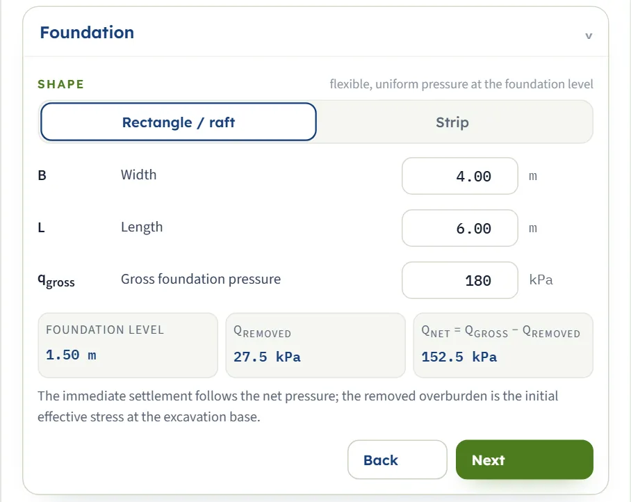
| Field (unit) | Starting value |
|---|---|
| Shape | Rectangle / raft |
| B, width (m · ft) | 4.00 |
| L, length (m · ft) | 6.00 (rectangle only) |
| qgross, gross pressure (kPa · t/m² · ksf) | 180 |
Analysis Settings
Where the compressible zone ends, and the slice thickness. The ? beside the title opens a window that explains the influence depth with a sketch. Influence depth (Δσ = p · q) sums the settlement down to the depth zlim where the stress increase under the centre has fallen to the share p of q; Bottom of the profile sums it down to the last layer, as for a rigid base right below. Three read-outs give the Calculation depth zlim, the depth below the foundation level and where the soil profile ends, and a note under them says what applies.
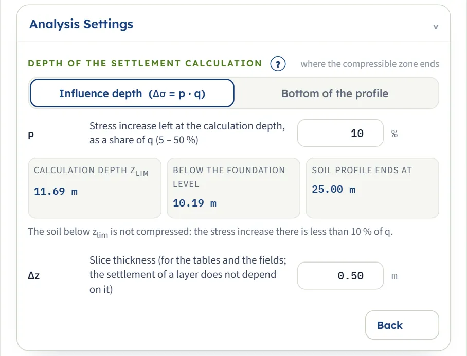
| Field (unit) | Starting value |
|---|---|
| Depth rule | Influence depth |
| p (%) | 10 (from 5 to 50; a typed value outside is brought back into this range) |
| Δz (m · ft) | 0.50 (from 0.05 to 2) |
The slice thickness Δz only sets how finely the layers are divided for the tables and the colour bands. Each layer is cut into the least number of equal slices not thicker than Δz; the settlement of a layer does not depend on it (Δz = 0.25 and 1.0 m give the same 24.1 mm as the starting 0.5 m).
Typed values that are brought into range
Several boxes keep a value inside its range instead of refusing it: p below 5 or above 50 becomes 5 or 50; Δz above 2 becomes 2; a width or length below 0.1 becomes 0.10; a negative pressure becomes 0; a negative water depth becomes 0.00. An empty box takes back its previous value. The inputs of an analysed model are locked until you press Edit inputs.
Choosing the options
Influence depth or bottom of the profile
The stress increase under a foundation falls with depth but never reaches zero, so the sum needs a lower end.
- Influence depth (the starting rule) stops where Δσz has fallen to p of q under the centre. A smaller p goes deeper and adds a little more. If the soil profile is shorter than that depth, the last layer is taken to continue down to it with the same properties; if it is longer, the soil below is not compressed.
- Bottom of the profile sums the settlement down to the bottom of the last layer. Use it when a rigid stratum (rock, very dense gravel) lies right below the profile: the settlement stops there, whatever the stress increase left at that depth. The note under the read-outs gives that share, for the example 2 % of q.
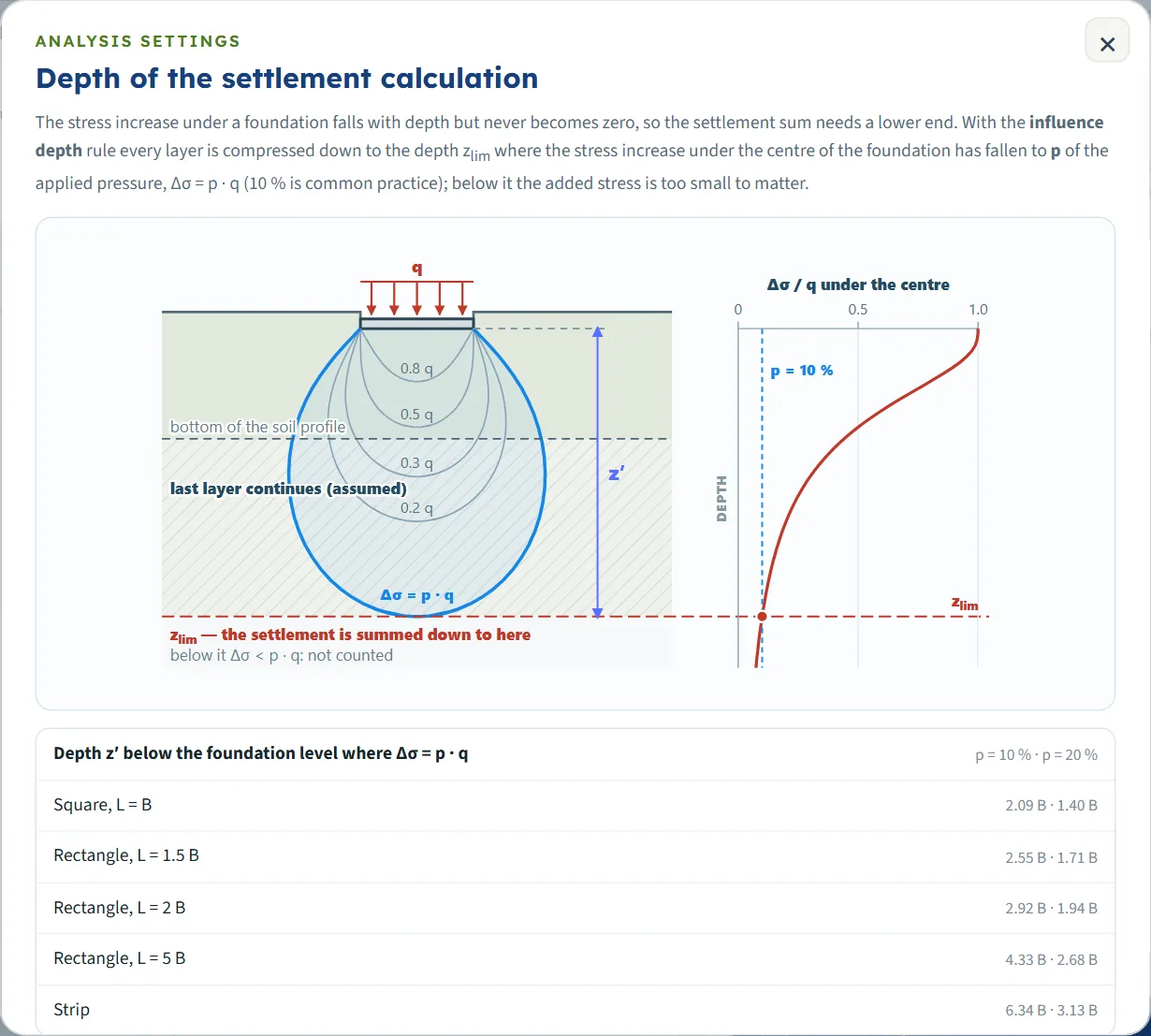
Rectangle or strip
Choose Strip for a long foundation (a wall footing, a long raft): the length box disappears and the module uses the plane limit of the factors. Its stress bulb goes deeper, so the influence depth is greater: for the example the strip gives zlim = 26.86 m against 11.69 m, and the profile (25 m) is continued below its bottom with the last layer’s properties. The result card then says Edge instead of Corner.
Excavation yes or no
The excavation lowers the foundation level and takes off the soil weight: with No the whole qgross loads the soil (180 kPa for the example, against a net 152.5 kPa), and the settlement is 29.8 mm against 24.1 mm. Use Yes when the foundation really sits at the base of an excavation.
Centre, corner and rigid
A flexible foundation settles most at the centre and least at the corner. The module gives both, and their difference. A rigid foundation is taken at 0.93 times the flexible centre settlement. Read the one that matches the stiffness of your foundation, or the corner and centre as bounds.
Analyze and read the results
Press Analyze. The bar briefly counts through four steps (net pressure, calculation depth, Steinbrenner factors, layer settlements) and then reads Analysed — 2 layers, 21 slices down to 11.69 m, followed by “The inputs are locked. Edit inputs clears the results; the unit system can still be changed.” A message “Analysed — the settlement of the section; see also Contours and the Results tab.” appears for a moment. The module stays on the Model tab, switches the drawing to the Settlement view, and the numbers are on the Results tab. If the run has a caution, the Warnings window opens by itself (see Messages).
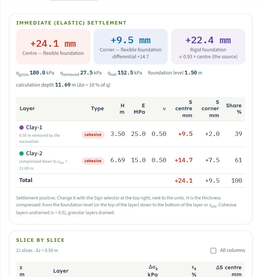
The cards and the table by layer
| Card | Meaning | Example |
|---|---|---|
| Centre — flexible foundation | The settlement under the centre of the flexible foundation. | 24.1 mm |
| Corner — flexible foundation (Edge for a strip) | The settlement at the corner, with the differential (centre − corner) beneath. | 9.5 mm; differential 14.7 |
| Rigid foundation | 0.93 times the flexible centre settlement. | 22.4 mm |
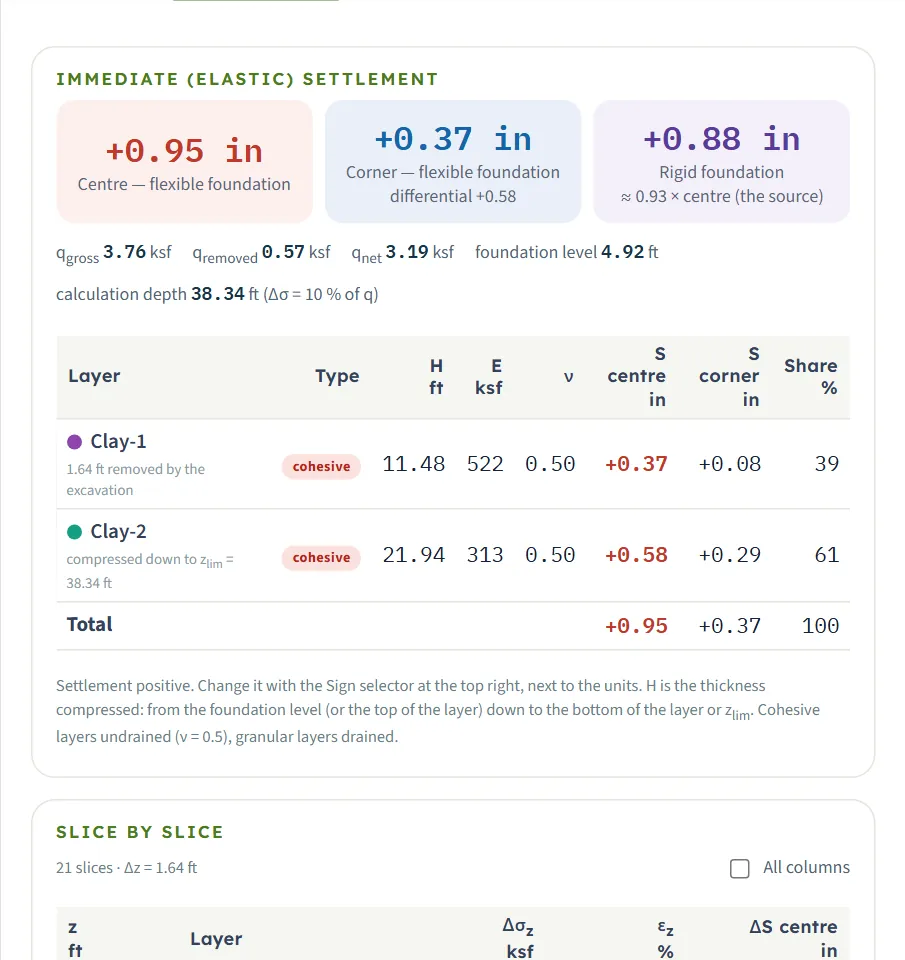
Under the cards a line gives qgross, qremoved, qnet, the foundation level and the calculation depth with the rule used. The table lists every layer that is compressed: its type, the thickness H compressed (from the foundation level or the top of the layer down to its bottom or zlim), E, ν, the settlement at the centre and at the corner, and its share of the total. A note under the name tells when part of a layer is removed by the excavation (Clay-1: “0.50 m removed by the excavation”), when it is compressed only down to zlim (Clay-2), or when the profile has been continued (“continued from … to … (assumed)”).
In the example Clay-1 gives 9.5 mm (39 %) and Clay-2 14.7 mm (61 %) at the centre.
Slice by slice
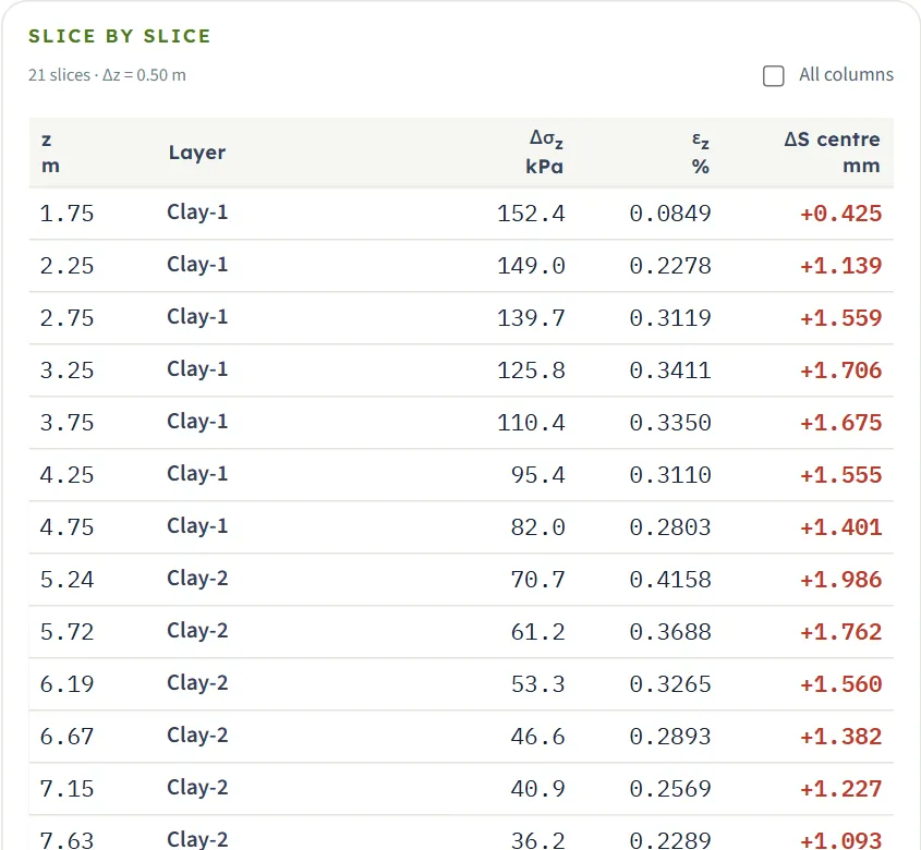
The second table gives each slice: its mid-depth z, the layer, Δσz, εz (in %) and the centre settlement ΔS. All columns adds the thickness, E, ν and the corner settlement. Click a row to see the working of that slice on the Calculations tab.
Units and sign
Changing the unit system or the sign convention after Analyze re-states the cards, tables, drawings and report without a new run. With Sign: settlement − every displacement is written with the opposite sign (the vertical displacement positive upward); strains and stresses keep compression positive. In US the starting example gives +0.95 in at the centre, 0.37 in at the corner and 0.88 in for the rigid foundation, the same 24.1, 9.5 and 22.4 mm.
The Calculations tab, the report and the Theory tab
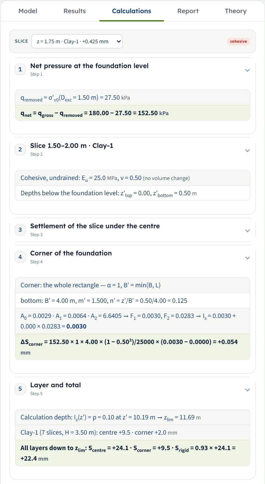
The Calculations tab writes out the working of one slice at a time. Choose the slice in the Slice list (or click a row in the Results tab). There are five steps, each with its own equations and your numbers; steps 1, 2, 3 and 5 are open and step 4 is closed until you open it:
- Net pressure at the foundation level: qremoved = σ′v0(Dexc) and qnet = qgross − qremoved (for the example 27.50 and 152.50 kPa).
- The slice: its depths, its Eu and ν = 0.50 (“no volume change”), and its depths below the foundation level, z′top and z′bottom.
- Settlement of the slice under the centre: B′, m′ and n′ for the top and bottom of the slice, the terms A0, A1, A2, the factors F1 and F2, Is, and ΔScentre.
- Corner of the foundation (Edge for a strip): the same working for the corner, with α = 1 and B′ = min(B, L), or α = 2 for the edge of a strip.
- Layer and total: the calculation depth, the layer of the slice with its settlements, and the totals Scentre, Scorner and Srigid = 0.93 × Scentre.
With Sign: settlement − a note says the derivation is written in the classical convention (settlement +) while the results, tables and drawings follow the sign you chose. Before Analyze the tab says “Press Analyze on the Model tab first.”
The report
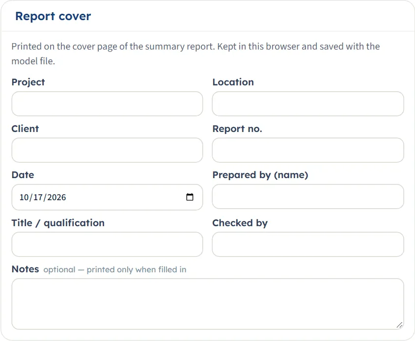
In Report fill in the cover: Project, Location, Client, Report no., Date, Prepared by (name), Title / qualification, Checked by and optional Notes (printed only when filled in). They are kept in this browser and saved with the model file. After Analyze Save as PDF (it opens a print window: choose “Save as PDF” in the print dialog) and Download Word (.docx) are available; before it they are greyed out. The preview below is the report itself.
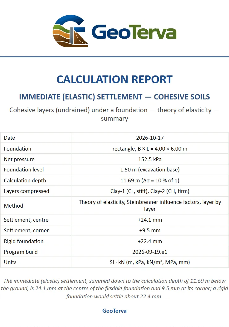
The report has eight parts: 1 Introduction and scope, 2 Soil profile and elastic parameters, 3 Foundation, loading and calculation depth, 4 Method and assumptions, 5 Immediate settlement, 6 Slice by slice, 7 Summary and 8 References. When the run carries a caution a part 7 Warnings is added and the last two become 8 and 9. It carries the section and the stress and settlement colour-band drawings and states the units with the conversion constants.

The Theory tab
The Theory tab has thirteen sections, each opened from the contents list at its top: Scope; Theory of elasticity; Steinbrenner’s influence factors; Layered profile; Cohesive layers; Net pressure; Depth of the settlement calculation; Flexible and rigid foundations; Embedment; Colour-band fields; Sign convention and assumptions; Outside the scope; and References.
Worked example: the module’s own example
The module opens on this example, so you can follow the numbers on your screen.
| Section | Input |
|---|---|
| Soil profile | Fill 0–1 m (γ 18.0 / γsat 19.0), Clay-1 1–5 m (19.0 / 19.5), Clay-2 5–12 m (18.5 / 19.0), Clay-3 12–25 m (19.5 / 20.0) |
| Elastic parameters | Eu: fill 8, Clay-1 25, Clay-2 15, Clay-3 45 MPa; ν = 0.5 |
| Groundwater | zw = 2.5 m |
| Excavation | Yes, Dexc = 1.5 m |
| Foundation | Rectangle, B = 4 m, L = 6 m, qgross = 180 kPa |
| Analysis Settings | Influence depth, p = 10 %, Δz = 0.5 m |
Step 1: the net pressure
The excavation (1.5 m) lies above the water table (2.5 m): qremoved = 18.0 × 1.0 + 19.0 × 0.5 = 27.5 kPa, and qnet = 180 − 27.5 = 152.5 kPa. The fill (0–1 m) and the top 0.5 m of Clay-1 are above the foundation level, so they are not compressed.
Step 2: the calculation depth
For a 4 × 6 m rectangle the stress increase under the centre falls to 10 % of q at z′ = 10.19 m below the foundation level, so zlim = 1.5 + 10.19 = 11.69 m. That is inside Clay-2; Clay-3 below is not compressed. The compressed thickness is 3.50 m of Clay-1 (1.5 to 5.0 m) and 6.69 m of Clay-2 (5.0 to 11.69 m): 21 slices in 2 layers.
Step 3: a slice by hand
For the first slice (1.50–2.00 m) of Clay-1: B′ = B/2 = 2.00 m, m′ = 1.500 and n′ = 0.50 / 2.00 = 0.250 at its bottom; F1 = 0.0116 and F2 = 0.0508, and since ν = 0.5 the term with F2 drops out: Is = 0.0116 (and 0 at its top). So ΔS = 152.5 × 4 × 2.00 × (1 − 0.5²) / 25000 × 0.0116 = +0.425 mm, the first entry of the slice table.
Step 4: the layers and the totals
Adding the slices gives Clay-1 9.5 mm and Clay-2 14.7 mm, a centre settlement of 24.1 mm. The same sums at the corner give 2.0 + 7.5 = 9.5 mm, and the rigid foundation 0.93 × 24.1 = 22.4 mm. These are the numbers on the Results tab. An independent numerical integration of the strains of a point load over the loaded area and the depth gave 9.46 mm and 14.65 mm at the centre for the two layers, the same to the digit shown.
The same model in the other units
Switch to SI · tf: the cards stay in mm (24.1, 9.5, 22.4) and the pressures read qgross 18.4, qremoved 2.8 and qnet 15.6 t/m². In US: +0.95 in, 0.37 in and 0.88 in; qgross 3.76 ksf, qnet 3.19 ksf, the foundation level 4.92 ft and zlim 38.34 ft.
How each input changes the answer
Each row changes one thing in the example (B × L = 4 × 6 m, qgross = 180 kPa, Dexc = 1.5 m, zw = 2.5 m, p = 10 %, Eu = 25 and 15 MPa in the two compressed layers, γ as in the example) and runs the module again. The numbers are the ones the module gives. Settlements in mm.
| Change | Centre | Corner |
|---|---|---|
| The example qnet = 152.5 kPa · zlim = 11.69 m | 24.1 | 9.5 |
| Eu of Clay-2 = 30 MPa (was 15) Clay-2’s share halves. qnet = 152.5 kPa · zlim = 11.69 m | 16.8 | 5.7 |
| Eu of Clay-2 = 7.5 MPa Clay-2’s share doubles. qnet = 152.5 kPa · zlim = 11.69 m | 38.8 | 16.9 |
| Eu of Clay-1 = 50 MPa (was 25) qnet = 152.5 kPa · zlim = 11.69 m | 19.4 | 8.5 |
| qgross = 100 kPa qnet = 72.5 kPa · zlim = 11.69 m | 11.5 | 4.5 |
| qgross = 300 kPa qnet = 272.5 kPa · zlim = 11.69 m | 43.1 | 16.9 |
| B = 2 m a narrower foundation: shallower influence depth. qnet = 152.5 kPa · zlim = 8.51 m | 13.9 | 5.3 |
| B = 5 m qnet = 152.5 kPa · zlim = 12.92 m | 27.5 | 10.5 |
| L = 4 m (square) qnet = 152.5 kPa · zlim = 9.85 m | 19.0 | 7.5 |
| L = 12 m qnet = 152.5 kPa · zlim = 15.52 m | 30.0 | 10.7 |
| Strip, B = 4 m the last layer is continued below 25 m. qnet = 152.5 kPa · zlim = 26.86 m | 32.7 | 23.2 |
| Excavation: No qnet = 180. qnet = 180.0 kPa · zlim = 10.19 m | 29.8 | 10.7 |
| Dexc = 3 m a deeper excavation removes more weight. qnet = 128.7 kPa · zlim = 13.19 m | 22.2 | 8.1 |
| zw = 0.5 m water above the base of the excavation: less weight is removed. qnet = 161.6 kPa · zlim = 11.69 m | 25.5 | 10.0 |
| zw = 8 m the water table is below the excavation: same answer as 2.5 m. qnet = 152.5 kPa · zlim = 11.69 m | 24.1 | 9.5 |
| p = 20 % qnet = 152.5 kPa · zlim = 8.32 m | 19.4 | 6.4 |
| p = 5 % qnet = 152.5 kPa · zlim = 16.28 m | 25.4 | 10.5 |
| Bottom of the profile down to 25 m. qnet = 152.5 kPa · zlim = 25.00 m | 26.3 | 11.3 |
| Δz = 0.25 m more slices, the same settlement. qnet = 152.5 kPa · zlim = 11.69 m | 24.1 | 9.5 |
| Clay-3 deleted, Clay-2 ends at 9 m Clay-2 is continued to 11.69 m: the same as the example. qnet = 152.5 kPa · zlim = 11.69 m | 24.1 | 9.5 |
| The same, with Bottom of the profile the sum stops at 9 m. qnet = 152.5 kPa · zlim = 9.00 m | 20.6 | 7.1 |
What the rows show
- The modulus divides the settlement of its layer: doubling Eu of Clay-2 takes its part from 14.7 mm to 7.3 mm.
- The pressure acts on the net pressure: 100 kPa gives qnet = 72.5 kPa, and the settlement is proportional to it (11.5 mm; 300 kPa gives 43.1 mm).
- The size of the foundation changes the stress bulb and so the influence depth as well: a wider or longer foundation settles more and goes deeper.
- The excavation and the water table act through the net pressure only: a water table below the base of the excavation (8 m) gives exactly the example’s answer.
- The depth rule changes how much of the profile is counted: a smaller p counts more.
- The slice thickness does not change the answer.
Messages: stops and cautions
Stop: the module cannot analyse
When an input needed for the calculation is missing, Analyze shows a window titled Cannot analyse — 1 input error (or 2 input errors, and so on) that lists them, and nothing is calculated. The bar stays at Not analysed. Through the boxes of the Model tab the stop that can arise is a missing modulus, because the other boxes are brought into range or keep their previous value:
| When | Message and what to do |
|---|---|
| A layer that is compressed has an empty or zero Eu | “Clay-2 (CH, firm): Eu is missing — needed below the foundation level.” The layer is named; enter the modulus. Each layer gives its own line. |

Caution: the module analyses and says what to look at
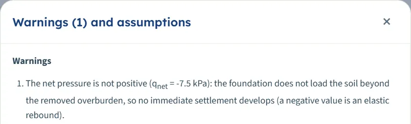
A caution does not stop the analysis. The bar reads Analysed — … — 1 warning (or warnings), the Results and Report tabs show a strip with the first warning and a Warnings (N) button, and the Warnings window opens by itself after Analyze. It lists the warnings and, below them, the assumptions of the analysis. Warnings (N) in the bar opens it again.

| When | Message |
|---|---|
| qgross is not larger than the removed overburden (20 kPa against 27.5 kPa; also 0 kPa) | “The net pressure is not positive (qnet = -7.5 kPa): the foundation does not load the soil beyond the removed overburden, so no immediate settlement develops (a negative value is an elastic rebound).” The settlement is then zero or negative. |
| The excavation is as deep as the profile or deeper (25 m, 30 m; with one layer left, 1 m) | “The excavation reaches the bottom of the soil profile (25.00 m).” The layers above are removed; the last layer is continued down to the calculation depth. |
| No soil lies between the foundation level and the calculation depth (excavation 25 m and Bottom of the profile) | “No soil between the foundation level and the calculation depth: nothing settles.” |
Assumptions that are stated, not cautions
The assumptions list also says, in words, what the module did with your profile: that a layer above the foundation level was removed by the excavation, that the part of a layer below zlim is left out, and that the last layer was continued when the profile ended above zlim: “The soil profile ends at 9.00 m, above zlim: Clay-2 (CH, firm) is taken to continue down to 11.69 m with the same properties. Choose "Bottom of the profile" when a rigid stratum lies right below the profile.” This also shows in the note of Analysis Settings and in the layer table of the results.
Good practice and common mistakes
- Think about Eu first. It sets the answer layer by layer, and a typical range spans a factor of several. Split a layer whose stiffness changes with depth.
- This is the immediate settlement. Clay then consolidates; add that from Consolidation settlement, or use Settlement 2D for the total of a profile with clay and sand.
- Use this module for clay and silt layers. A layer of sand or gravel in the profile belongs to the granular module or to Settlement 2D, which treat it drained.
- Enter the gross pressure at the foundation level, and the excavation depth as the depth of that level. The module takes the net pressure for you.
- Check the calculation depth. Read the three read-outs in Analysis Settings. If the profile ends above zlim and you know a rigid stratum is there, choose Bottom of the profile.
- Read centre and corner as bounds for a flexible foundation, and the rigid value for a stiff slab.
- Keep the sign convention in mind when comparing with other programs’ output: the Sign selector in the header changes every displacement shown.
- Save the model with Save to file or Quick Save for the project record; the browser keeps only the last model.
Frequently asked questions
What does this module calculate?
The immediate settlement of a flexible rectangular or strip foundation on clay and silt layers that deform undrained: the vertical strain, with Eu and ν = 0.5, is added up layer by layer with the influence factors of Steinbrenner, down to the calculation depth. It gives the centre, the corner (edge) and the rigid-foundation settlement.
Why is ν fixed at 0.5?
Right after loading a saturated clay deforms without a change of volume, which is ν = 0.5. The later volume change, the consolidation, is not part of this module; Consolidation settlement computes it and Settlement 2D adds the two.
What is the calculation depth?
The depth zlim down to which the settlement is summed. With the influence-depth rule it is where the stress increase under the centre has fallen to p of the pressure (10 % to start with); with Bottom of the profile it is the bottom of the last layer. For the example zlim = 11.69 m.
Why do the first layers get no modulus box?
A layer above the foundation level is removed by the excavation, and a layer below the calculation depth is not compressed, so neither needs a modulus. The table says so in their rows.
What if my profile is shorter than the calculation depth?
With the influence-depth rule the last layer is taken to continue down to zlim with its own properties, and the module says so. If a rigid stratum lies right below your profile, choose Bottom of the profile instead.
How is the rigid foundation value found?
As 0.93 times the settlement at the centre of the flexible foundation. For the example 0.93 × 24.1 = 22.4 mm.
Why does the water table matter if the soil is clay?
It enters through the effective overburden removed by the excavation. With the excavation above the water table, moving the table deeper changes nothing; raising it above the foundation level reduces the removed weight and raises the net pressure.
Can I drag the foundation or the layers on the drawing?
No. The drawings are read-only; change the values in the Model tab. The Show chips and the Field buttons change what is drawn.
Does the module remember my inputs?
Yes. Every change is kept in this browser, and the page opens on the last model, analysed if it was. Reset to defaults returns to the example. Save to file and Quick Save keep versions you can come back to; the units and the sign convention are remembered as well.
Why is the settlement negative or zero in my run?
The gross pressure does not exceed the removed overburden, so the net pressure is not positive. The module warns “The net pressure is not positive” and shows the elastic rebound as a negative value. Check the pressure and the excavation depth.
What does the sign selector do?
It shows settlement as positive (the starting choice) or as negative, the vertical displacement being positive upward. It changes the numbers shown in results, tables, drawings and report, and nothing in the calculation.
What does the report contain?
A cover with your project details and a summary, then eight parts: introduction and scope, soil profile and elastic parameters, foundation and calculation depth, method and assumptions, the immediate settlement, every slice, a summary and references, with the section and the colour-band drawings. It is saved as PDF or Word after Analyze.