

What the module calculates
Braced cut in sand designs the bracing of a strutted excavation in sand: sheeting on both sides, wales along the sheeting and struts across the cut. It draws Peck’s apparent pressure envelope, gives the load of every strut for any number of strut levels from 2 to 15, finds the moments in the sheeting and in the wales, and verifies the sheeting, the wales and the struts to EN 1993-1-1 or AISC 360-22. When the water table stands above the base of the cut it adds the hydrostatic pressure on the wall and checks the base against piping.
The envelope is one uniform pressure over the full depth of the cut:
where σ′v(H) is the effective vertical stress at the base of the cut. The sheeting is then treated as a beam on the struts, hinged at the struts according to the hinge convention you choose; each strut load is the reaction per metre of wall times the horizontal spacing, P = R × s.
What you can describe
- A cut of depth H and width B, with the sheeting embedded d below the base.
- One to ten layers of sand, each with its moist and saturated unit weight and friction angle.
- Two to fifteen strut levels at depths you give or drag, at a horizontal spacing s.
- The water table below the base or at a depth zw, with the hydrostatic pressure on the wall switched on or off.
- A uniform surcharge beside the cut.
- The sheeting by its section modulus; the wale and the strut by their numbers or from a catalogue of steel sections; steel grade S235, S275, S355 or typed.
- The piping check with the exit gradient from a flow net, from Harr’s charts or given.
Which module for which cut
- Sand throughout: this module. Clay throughout, with the check against bottom heave: Braced cut in clay. Sand over clay: Braced cut in sand over clay.
- The family overview: Braced cuts.
- The Rankine coefficient on its own: Rankine. A wall held by anchors or by its embedment alone: Sheet-pile walls.
Before you start: what you need
Have these ready:
| What | Notes |
|---|---|
| The sand Boring logs and tests | For each layer from the top: thickness (not the last), moist unit weight, saturated unit weight (needed with a water table) and the friction angle φ′, from 15° to 45°. |
| The cut Your design | Depth H, width B, the embedment d of the sheeting, and, for the drawing, the plan length L and the depth T to an impervious layer. |
| The water Groundwater readings | The depth zw of the water table behind the sheeting, or that it lies below the base. |
| The bracing Your design | The depth of each strut level and the horizontal spacing s. |
| The members The maker’s tables | Steel grade and section modulus of the sheeting per metre of wall; of the wale; area and weak-axis second moment of the strut, or their catalogue sections. |
| The piping data, if the water is above the base | Head loss h, Nd and a of a flow net, or a chart value, or the exit gradient itself; the critical gradient icr. |
Quick start in eight steps
- Open the module and choose the units
Open Braced cut in sand from the Braced Cuts family. Pick SI · kN, SI · tf or US in the header; you can change it at any time, even after Analyze.
- Describe the sand
In Soil layers change the first layer, Sand, or fill the New layer form and press + Add layer. The last layer runs on below the cut.
- Set the water
In Groundwater choose Below the base or Present and type the depth zw.
- Give the cut and the surcharge
In Cut geometry type H, B, d and, if you wish, L and T. In Surcharge add a uniform load if there is one.
- Place the struts
In Struts type the spacing s and the depth of each level, or drag the levels on the drawing. + Add a strut level and Remove the last strut change the number.
- Give the members
In Sections choose the steel grade and the section of the sheeting, the wale and the strut. In Analysis settings choose the hinge convention and the design code.
- Press Analyze
Press Analyze at the foot of the Model tab. The bar reads Analysed — the braced cut calculated and the inputs lock.
- Read the answer and take the report
The Results tab gives the diagrams, the strut loads, the moments and the verdict on every member; Calculations writes the working; Report saves a PDF or Word file.
The screen: Section, 3D and the handles
The layout is the one every GeoTerva module shares (workspace guide): the drawing on the left, the tabs Model, Results, Calculations, Report and Theory on the right. The drawing has two views:
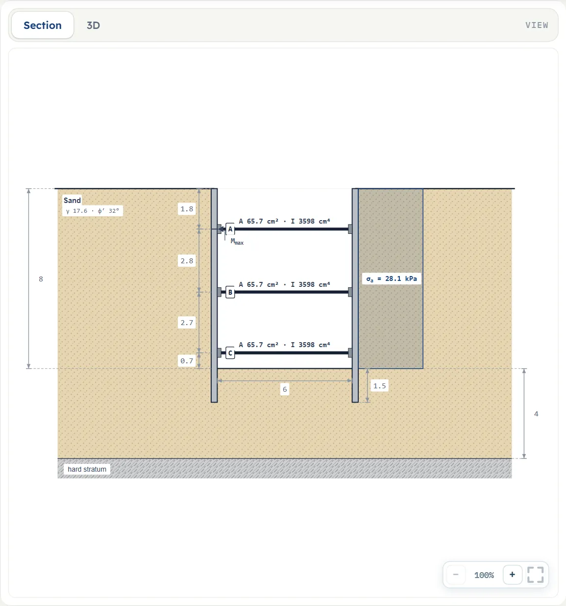
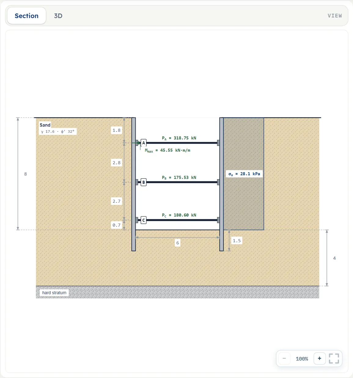
- Section is the cut with its layers, the sheeting, the struts and wales, the apparent-pressure envelope and the dimensions. It follows your inputs. After Analyze it adds the strut loads, the maximum sheeting moment Mmax and the pressures; a member is green where it carries its force and red where it does not.
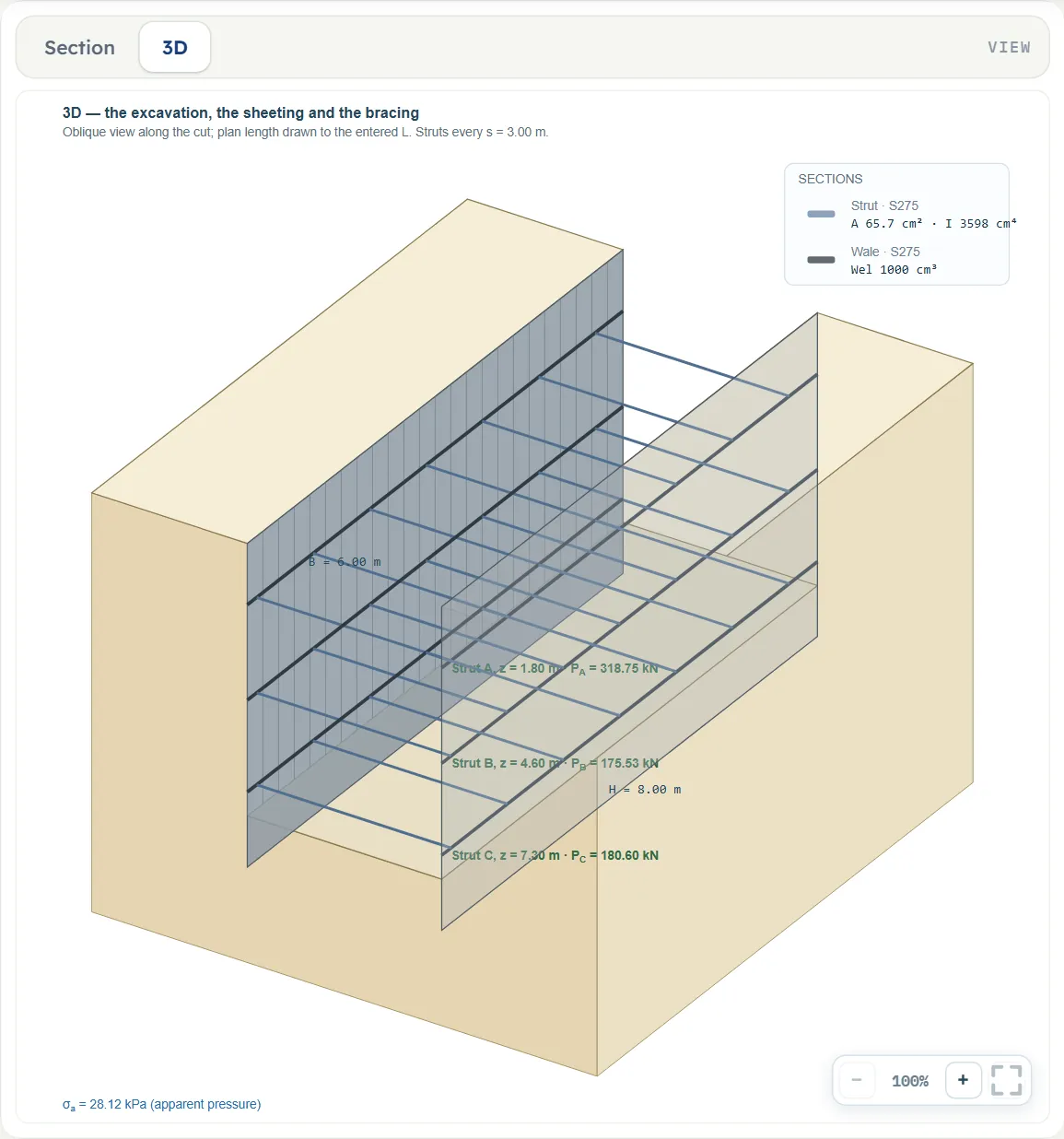
- 3D is an oblique view of the excavation: the sheeting on both sides, the wales and the struts at their spacing, a legend of the sections, and after Analyze the load of each strut level.
Zoom and Show chips
There are no Show chips: the drawing shows everything. Each view has −, a percentage and + at the lower right and a button that fits the whole drawing in the pane.
Handles on the drawing
- Before Analyze you can drag a strut up or down; the field of that strut in the Model tab follows. The drag stops at 0.1 m below the surface and at 0.1 m above the base, so a dragged strut stays inside the cut; a level typed outside it stops the analysis (see Messages).
- Press a layer on the drawing and it opens in its form.
- After Analyze nothing can be moved and the inputs are locked; Edit inputs unlocks them and clears the results. The unit system can still be changed.
Entering the model, section by section
The Model tab has nine sections: Model data, Soil layers, Groundwater, Cut geometry, Surcharge, Struts, Sections, Piping and Analysis settings. Model data opens and closes on its own; the other eight sections work as an accordion, opening one closes the previous one; Next and Back walk you through them. Where a unit is given twice, such as m · ft, the units are those of SI and US, and the defaults are shown in SI.
Model data
The model name, Save to file…, Open file…, Quick Save… with its list, Load, Delete and Reset to defaults, as in the workspace guide. After Analyze these are locked until you press Edit inputs.
Soil layers
A New layer form over a table. Fill the form and press + Add layer: the layer goes to the bottom of the table (up to ten, with a counter). Press a row to change it in the form, which then offers Done and Delete layer; × removes a layer. The thicknesses add up from the ground surface; layers below the base of the cut are not used for the envelope. Several layers are reduced to one Ka by the rule in Analysis settings.
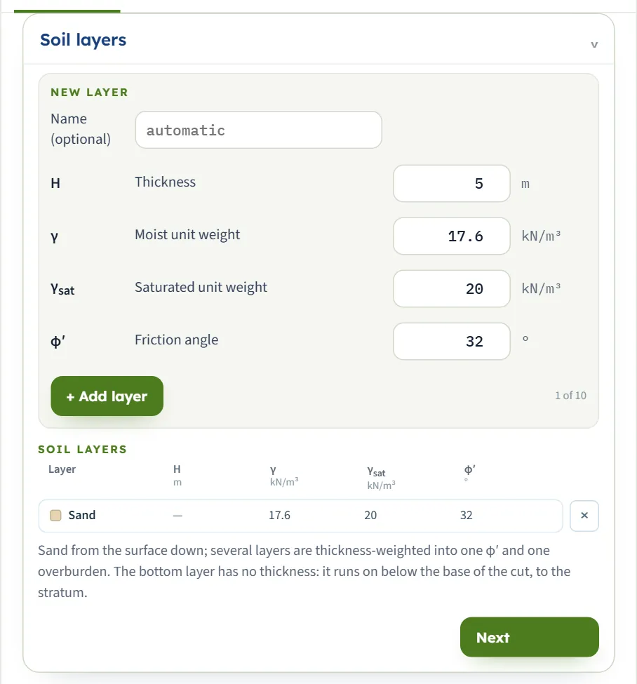
| Field | Default | What to enter |
|---|---|---|
| Name optional | automatic | Sand, or Sand-1, Sand-2 … when there are several. |
| Thickness H m · ft | 12 (first layer); 5 (new form) | At least 0.1 m. The last layer has none: it runs on below the cut, and its row shows a dash. |
| Moist unit weight γ kN/m³ · t/m³ · pcf | 17.6 | At least 1. Used above the water table. |
| Saturated unit weight γsat kN/m³ · t/m³ · pcf | 20 | At least 1; above 9.81 kN/m³ when there is a water table. |
| Friction angle φ′ ° | 32 | From 15° to 45°. |
Groundwater
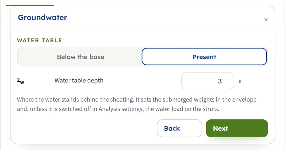
Water table: Below the base (default) or Present. With Present, type the depth zw (default 3 m, zero or more) below the ground surface; a water table above the base turns on the hydrostatic pressure and the piping check. Below the base the water has no effect on the envelope and the Notes say no piping check is needed.
Cut geometry
Impervious layer below the base: At a known depth (default) or None within reach.
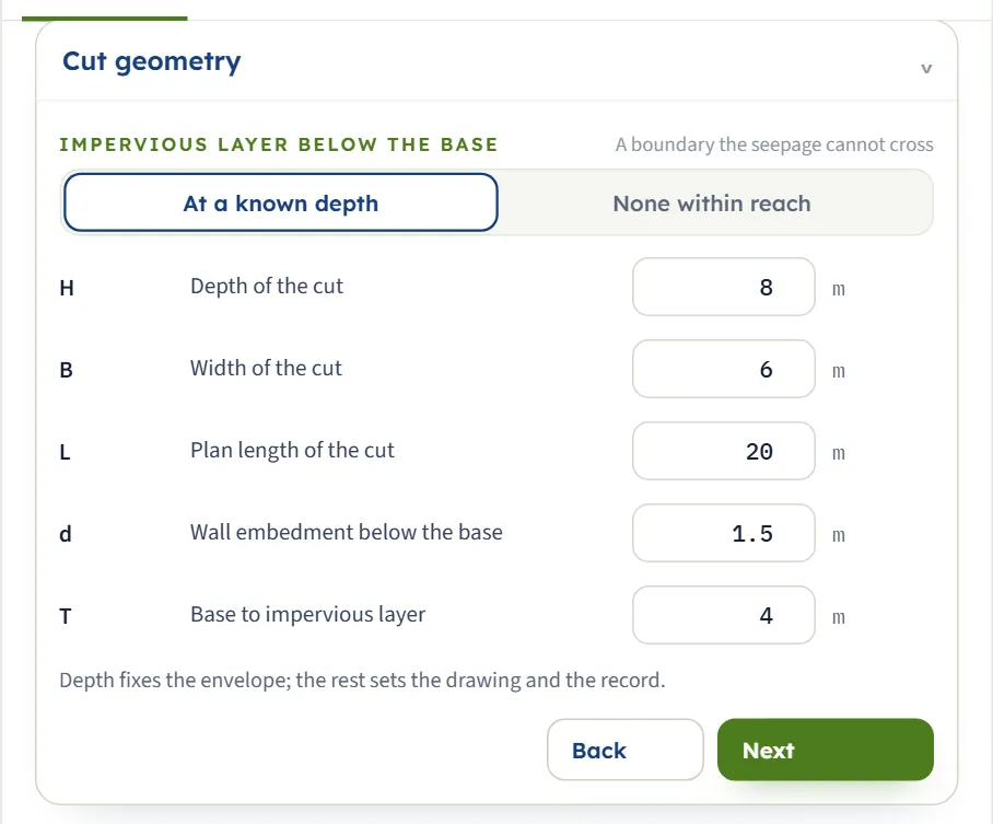
| Field | Default | What to enter |
|---|---|---|
| Depth of the cut H m · ft | 8 | At least 0.5 m. It fixes the envelope. |
| Width of the cut B m · ft | 6 | At least 0.5 m. It is the buckling length of the strut unless you type another. |
| Plan length L m · ft | 20 | At least 0.5 m; optional. It sets the drawing. |
| Embedment d m · ft | 1.5 | Zero or more. The sheeting below the base; it lengthens the seepage path. |
| Base to impervious layer T m · ft | 4 | Zero or more; optional, shown with a known depth. |
Surcharge
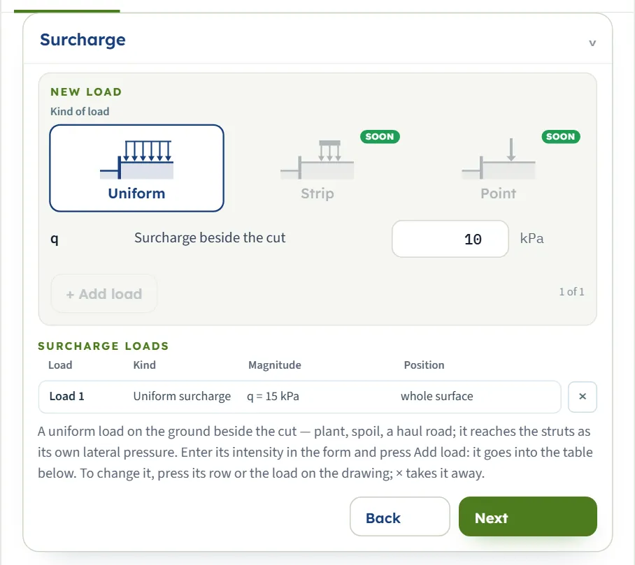
The form offers a Uniform load; Strip and Point stand beside it marked Soon and cannot be pressed. Type the intensity q (kPa, zero or more; the form opens with 10) and press + Add load: one load goes into the table (0 of 1). It acts as its own lateral pressure Ka q over the full depth and is not multiplied by 0.65. × removes it.
Struts
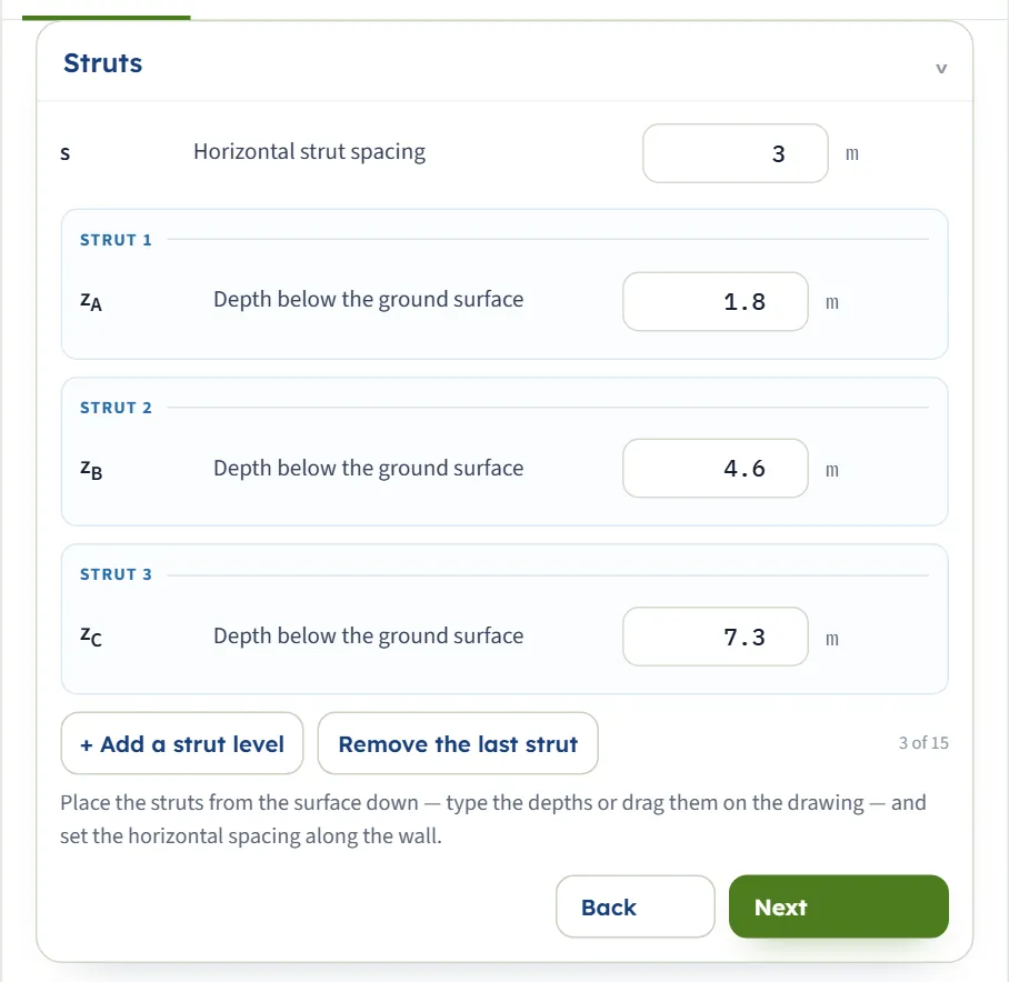
The horizontal spacing s (default 3 m, at least 0.5 m) and the depth of each level below the ground surface, A from the top (defaults 1.8, 4.6 and 7.3 m; each at least 0.1 m). + Add a strut level adds one up to 15, Remove the last strut takes one away down to 2; a counter shows “3 of 15”. Levels are analysed in order of depth, whatever order you type them in: with the second level typed at 1 m the module treats the struts as 1, 1.8 and 7.3 m (σa 28.12 kPa, Pmax 294.8 kN, Mmax 102.9 kN·m/m). A level at or below the base, or two levels at the same depth, stop the analysis.
Sections
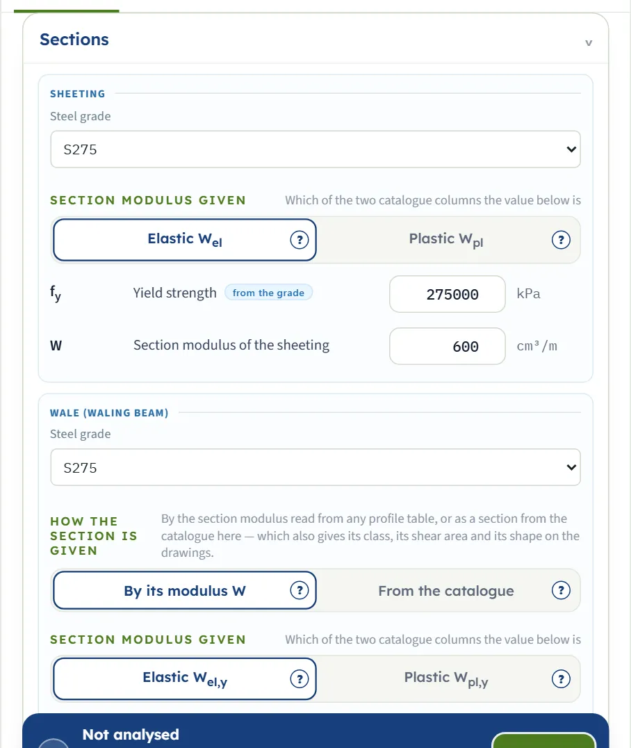
Three blocks, Sheeting, Wale (waling beam) and Strut, each with a Steel grade (S235, S275, S355 or Typed) and its fy, which follows the grade until you type your own.
- Sheeting: Elastic Wel or Plastic Wpl, and the modulus W per metre of wall (default 600 cm³/m, S275).
- Wale: By its modulus W (default, 1,000 cm³, elastic or plastic) or From the catalogue (IPE, HEA, HEB, HEM, UPN or a steel box with Width b, Depth h and Wall thickness t; the catalogue also gives its class and shear).
- Strut: By A and I (default A = 65.7 cm², Imin = 3,598 cm⁴, buckling curve c with EN 1993-1-1) or From the catalogue (CHS, SHS, RHS, IPE, HEA, HEB, HEM, UPN; tubes hot finished or cold formed).
- Buckling length Lb (the width of the cut until you type one), effective length factor K (1, from 0.5 to 2) and modulus E (210,000,000 kPa for EN 1993-1-1, 200,000,000 for AISC; from the design code).
Piping
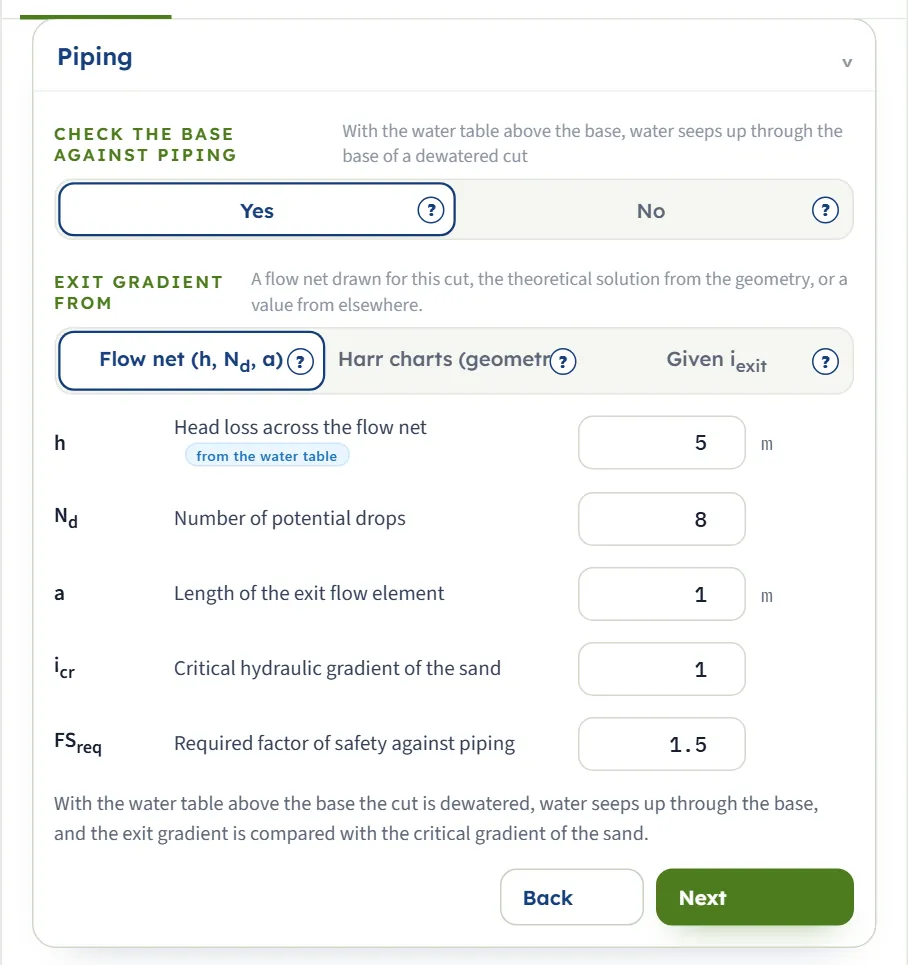
For a water table above the base: Check the base against piping Yes or No, and Exit gradient from Flow net (h, Nd, a), Harr charts (geometry) or Given iexit; each choice has a ? window.
| Field | Default | What to enter |
|---|---|---|
| Head loss h m · ft | 5 (from the water table) | The groundwater outside minus the level kept inside; it follows H − zw until you type one. |
| Potential drops Nd | 8 | At least 1. Flow net. |
| Exit element a m · ft | 1 | At least 0.05 m. Flow net. |
| Chart value L2 iexit / h | 0.5 | From 0.05 to 2. Harr. |
| Exit gradient iexit | 0.4 | At least 0.01. Given. |
| Critical gradient icr | 1 | From 0.5 to 1.5. |
| Required factor FSreq | 1.5 | From 1 to 3. |
Analysis settings
Layered profile — one Ka from: Weighted φ′ (default), Weighted Ka or Lowest φ′. Hinge convention: Auto, Interior struts, All but the top or Every strut. Design code: EN 1993-1-1 (Eurocode 3) with γF 1.35 (1 to 1.6), γM0 1.00 and γM1 1.00 (1 to 1.3), or AISC 360-22 with LRFD (γH 1.6, 1 to 2) or ASD. With a water table the Hydrostatic pressure on the wall choice also appears: Add γw (z − zw) or Envelope only.
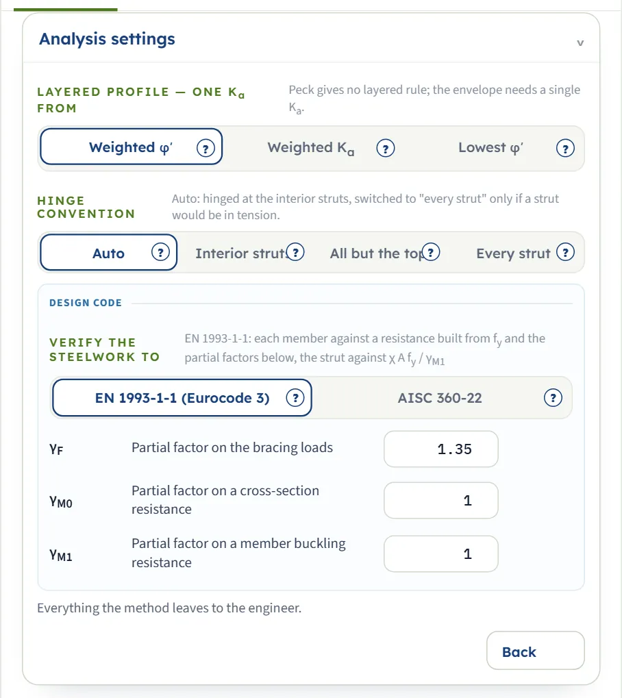
Choosing the hinge convention, the code and the water
Hinge convention
The sheeting is cut into pieces at its hinges; each piece is a determinate beam on the struts it holds. Auto and Interior struts hinge the sheeting at every strut except the top and the bottom one, and Auto switches to every strut only if a strut would be in tension. For the example with hinges at B the pieces are 0 to 4.6 m (struts A and B) and 4.6 to 8 m (B and C), and the strut loads are 318.75, 175.53 and 180.60 kN. Every strut gives 89.98, 77.33 and 57.64 kN/m, so the largest load is 270.0 kN; All but the top leaves the largest load at 318.8 kN.
Layered profile
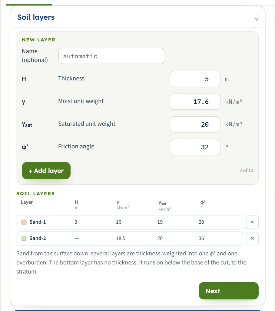
Peck gives one Ka, so a profile is reduced to one value. For a 3 m layer of 16 kN/m³ at 28° over sand of 18.5 kN/m³ at 36°: Weighted φ′ gives σa = 26.92 kPa, Weighted Ka 27.18 kPa and Lowest φ′ 32.97 kPa.
Water above the base
The overburden is taken effective below the water table, with γ′ = γsat − 9.81, and the hydrostatic triangle γw(z − zw) is added to the pressure on the wall. For the example with zw = 3 m: σa = 20.72 kPa, but the largest strut load rises from 318.8 to 376.7 kN. Envelope only leaves the water out; the module then raises a warning, because without the water the wall is loaded for less than ground and water together.
The code
EN 1993-1-1: the working values are factored once by γF, the sheeting and the wale are held to Mc,Rd = W fy / γM0 and the strut to Nb,Rd = χ A fy / γM1. AISC 360-22: LRFD factors the loads by γH and uses φ = 0.90; ASD uses the working loads against Rn / Ω with Ω = 1.67. For the example the section modulus the sheeting asks for is 223.6 cm³/m by EN 1993-1-1, 294.5 by LRFD and 276.6 by ASD.
Analyze and read the results
Press Analyze. The bar reads Analysed — the braced cut calculated, with Notes (n) or Warnings (n) and Edit inputs. The Model tab stays on screen: open Results. A window with warnings does not open by itself after Analyze in a clean case; with a failing member it opens at once.

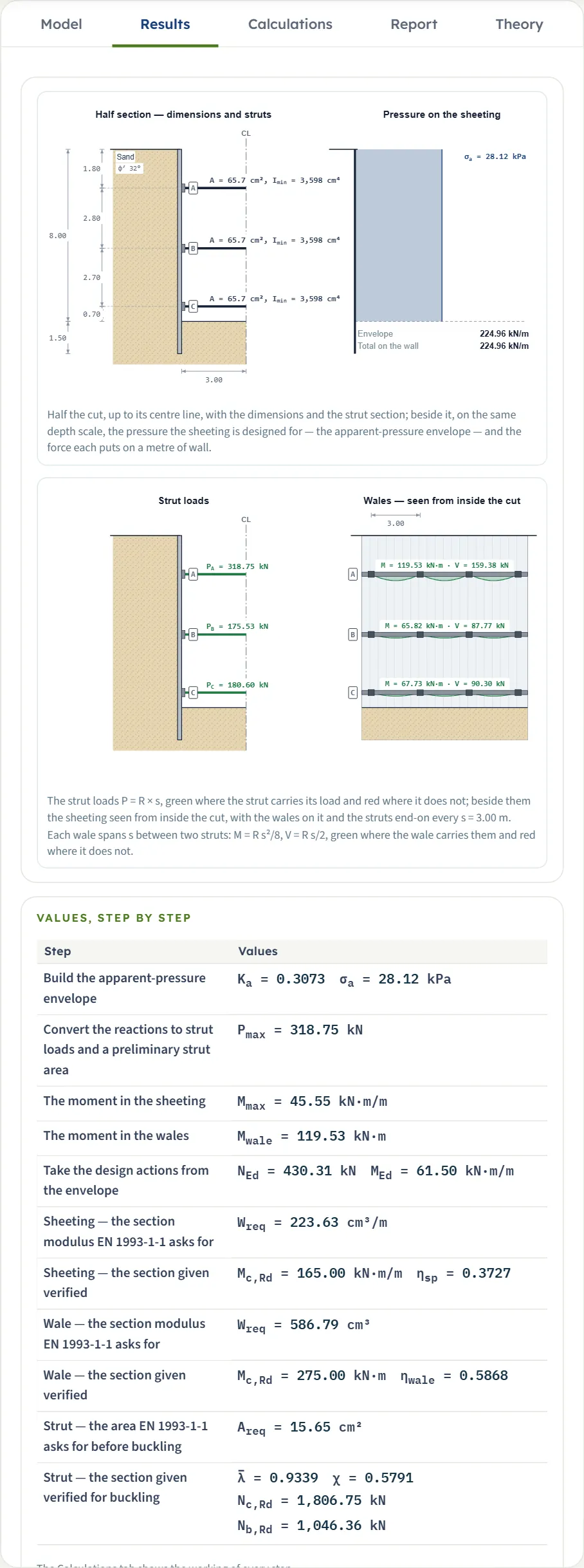
| Card | The example |
|---|---|
| Apparent pressure σa | 28.12 kPa |
| Largest strut load Pmax | 318.8 kN (strut A) |
| Maximum moment in the sheeting Mmax | 45.55 kN·m/m |
| Section modulus the sheeting needs Wreq,sp | 223.6 cm³/m |
| Sheeting ηsp | 0.3727 PASS |
| Wale ηwale | 0.5868 PASS |
| Strut (buckling) ηstrut | 0.4112 PASS |
With a water table above the base and the piping check on, an eighth card, Factor of safety against piping FSpiping, is added. The tables are Values, step by step, Beam pieces of the wall (load on the piece and reactions), Strut loads (z, R per metre, P = R × s and the preliminary area) and Wales, level by level (reaction, Mwale = R s² / 8 and the modulus asked for).
The verdict words
A utilisation reads PASS at 1 or less and FAIL above 1; very close to 1 it reads PASS — near capacity (the wale with only two struts, 0.9761). The piping card can also read NOT COMPARED, when the head loss differs from the one the wall was loaded with. The piping factor reads PASS at or above the required value and FAIL below it.
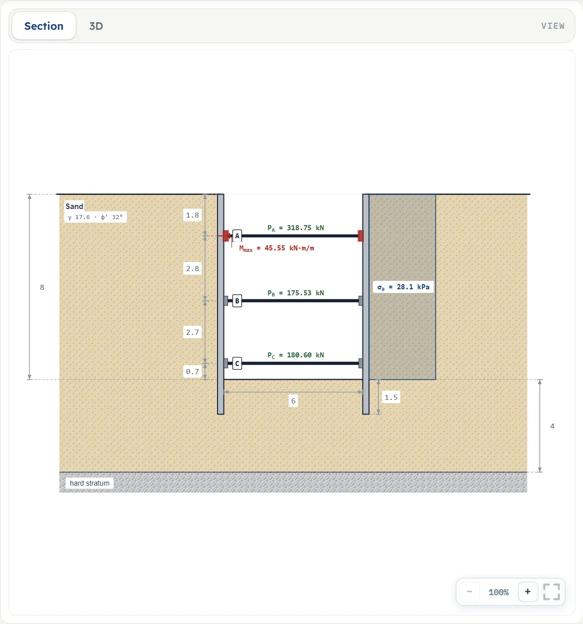
Using the numbers
- Strut loads are in kN (tf, kip) per strut; the reactions, and the moments in the sheeting, are per metre of wall; the wale moment is for one span s.
- σa and Mmax are working values; the factor of the code is applied once, in the design action.
- Changing the unit system re-states the cards, the tables, the working and the Section view (also before Analyze). The 3D view re-states the strut loads but keeps B, H, σa and the section legend in m, kPa and cm.
The Calculations tab, the report and the Theory tab
The Calculations tab starts with Given and what is sought and writes out the steps with your numbers. For the example they are: 1 Build the apparent-pressure envelope; 2 Idealise the sheeting and solve the strut reactions; 3 and 4 one step for each piece of the sheeting; 5 Take the yield strength of each member from its steel grade; 6 Convert the reactions to strut loads; 7 The moment in the sheeting; 8 The moment in the wales; 9 Take the design actions; 10 and 11 the sheeting, the modulus asked for and the section verified; 12 and 13 the same for the wale; 14 and 15 the strut, the area asked for and the buckling check. Notes and assumptions and the Answer close the tab. With the water above the base, steps for the hydrostatic load and for the piping check are added.
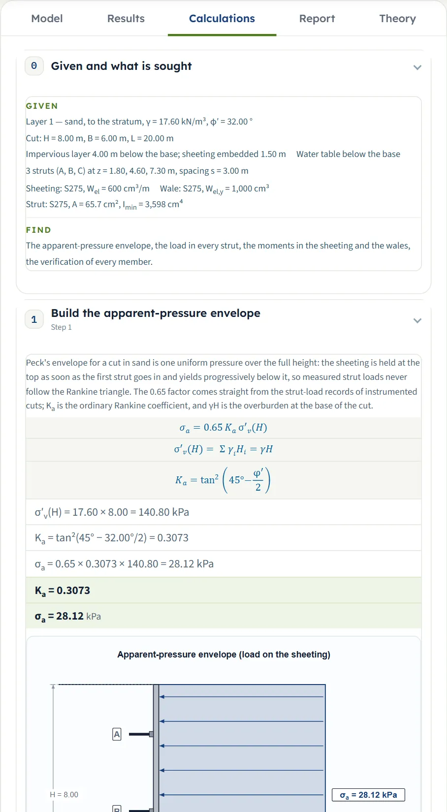
The Notes window
Notes (n) opens the assumptions of the run: that the sheeting is checked on the modulus given as the modulus of the whole wall; that the wale was verified on its modulus without its shear; that the class of a strut given by A and I was not computed; and that the bracing loads were factored by γF before the code check. With water above the base a note says the flow-net values must come from a net drawn for this cut. Warnings, when there are any, come first.
The report
In Report fill in the cover (project, location, client, report number, date, prepared by, title or qualification, checked by and notes); it is kept in this browser and saved with the model file. Save as PDF and Download Word (.docx) produce the report, which has seven parts: 1 Introduction and scope, 2 Input data, 3 Calculation (3.1 to 3.15; with water above the base two more steps appear: 3.2 Add the hydrostatic pressure and 3.10 Check the base against piping), 4 Results, 5 Assumptions and notes, 6 Summary and 7 References.
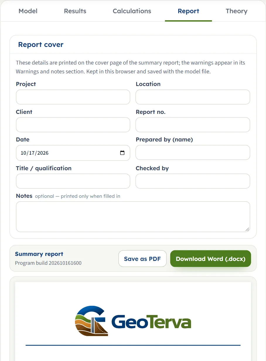
The Theory tab
The Theory tab has sixteen sections: The braced cut and its members; Why the pressure is not Rankine’s; Apparent pressure from measured strut loads; The envelope for sand; Water and a surcharge; Struts: from the envelope to the strut loads; Sheet piles; Wales; The members as they are given; Verifying the steel to EN 1993-1-1; Verifying the steel to AISC 360-22; The envelopes against real cuts; The base of a cut in sand: piping; What the method assumes, and what it leaves out; Worked example; References.
Worked example: the module’s own example
The module opens on this example. Inputs: one layer of sand, γ = 17.6 kN/m³, φ′ = 32°; water below the base; H = 8 m, B = 6 m, d = 1.5 m; struts A, B, C at 1.8, 4.6 and 7.3 m, s = 3 m; S275 members (fy = 275,000 kPa), sheeting Wel = 600 cm³/m, wale Wel = 1,000 cm³, strut A = 65.7 cm², Imin = 3,598 cm⁴; EN 1993-1-1, γF = 1.35.
The envelope
Ka = tan²(45° − 16°) = 0.3073; σ′v(H) = 17.6 × 8 = 140.80 kPa; σa = 0.65 × 0.3073 × 140.80 = 28.12 kPa.
The strut loads
Hinged at B, piece 1 runs from 0 to 4.6 m: W = 28.12 × 4.6 = 129.35 kN/m acting at 2.30 m, so RB = 129.35 × (2.30 − 1.80) / 2.80 = 23.10 kN/m and RA = 106.25 kN/m. Piece 2 runs from 4.6 to 8 m: W = 95.61 kN/m at 6.30 m, RC = 95.61 × 1.70 / 2.70 = 60.20 and RB = 35.41 kN/m. Strut B collects 23.10 + 35.41 = 58.51 kN/m. With s = 3 m: PA = 318.75 kN, PB = 175.53 kN, PC = 180.60 kN.
Sheeting, wale and strut
The largest sheeting moment is at A, Mmax = 28.12 × 1.8² / 2 = 45.55 kN·m/m. The wale at level A: Mwale = 106.25 × 3² / 8 = 119.53 kN·m. Design actions: NEd = 1.35 × 318.75 = 430.31 kN, MEd = 1.35 × 45.55 = 61.50 kN·m/m. The sheeting asks for Wreq = 61.50 / 275,000 = 223.63 cm³/m, and Mc,Rd = 600×10⁻⁶ × 275,000 = 165.00 kN·m/m gives ηsp = 0.3727. The wale: 1.35 × 119.53 = 161.37 kN·m, Wreq = 586.79 cm³, Mc,Rd = 275.00 kN·m, ηwale = 0.5868. The strut: Lcr = 1.00 × 6.00 = 6.00 m, Ncr = π² × 210,000,000 × 3,598×10⁻⁸ / 6² = 2,071.47 kN, λ̄ = √(65.7×10⁻⁴ × 275,000 / 2,071.47) = 0.9339, curve c gives χ = 0.5791 and Nb,Rd = 1,046.36 kN, so ηstrut = 430.31 / 1,046.36 = 0.4112 (rounded from 0.41125).
The piping check
With the water table at 3 m (everything else as above) the head loss follows H − zw = 5 m, iexit = 5 / (8 × 1) = 0.625 and FS = 1 / 0.625 = 1.600 PASS.
Other unit systems
The default example in US gives σa = 0.5873 ksf, Pmax = 71.65 kip, Mmax = 10.24 kip·ft/ft and Wreq = 4.160 in³/ft with the same utilisations; in SI · tf the same wall gives 2.870 t/m², 32.52 tf and 4.649 tf·m/m, with ηsp = 0.3731. Two checks with values typed in the other systems and recomputed by hand agree to within 0.2 %. In SI · tf the module carries Ka, σ′v and σa at the precision printed in the unit chosen (three digits in t/m²), so the printed numbers reproduce every load and the results differ from SI · kN by about 0.1 % (ηsp 0.3731 against 0.3727); US differs by less than 0.1 %:
- US. 112 / 125 pcf at 30°, H = 26 ft, B = 20 ft, s = 10 ft, struts at 6, 15 and 24 ft, 11 in³/ft, 61 in³, 10.2 in² and 86.4 in⁴: by hand σa = 0.6309 ksf, Pmax = 78.87 kip, ηsp = 0.4193; the module gives 0.6304 ksf, 78.80 kip and 0.4190.
- SI · tf. 1.8 / 2.0 t/m³ at 32°, geometry as the example: by hand 2.876 t/m², 32.60 tf and ηsp = 0.3737; the module gives 2.880 t/m², 32.64 tf and 0.3744.
How each input changes the answer
Each row changes one thing in the example (γ = 17.6 kN/m³, φ′ = 32°, water below the base, H = 8 m, s = 3 m, struts at 1.8, 4.6 and 7.3 m, S275, EN 1993-1-1 with γF = 1.35) and runs the module again. Each cell gives σa in kPa, Pmax in kN and Mmax in kN·m/m, then the utilisations of the sheeting, wale and strut.
| Change | Result |
|---|---|
| The example | 28.12 · 318.8 · 45.55 0.3727 · 0.5868 · 0.4112 |
| φ′ = 28° | 33.04 · 374.5 · 53.52 0.4379 · 0.6895 · 0.4832 |
| φ′ = 36° | 23.76 · 269.3 · 38.49 0.3149 · 0.4958 · 0.3475 |
| γ = 19 kN/m³ | 30.36 · 344.2 · 49.18 0.4024 · 0.6336 · 0.4440 |
| H = 9 m | 31.64 · 358.7 · 51.26 0.4194 · 0.6602 · 0.4627 |
| H = 7.5 m | 26.37 · 298.9 · 42.72 0.3495 · 0.5503 · 0.3857 |
| s = 2 m | 28.12 · 212.5 · 45.55 0.3727 · 0.2608 · 0.2742 |
| s = 4 m | 28.12 · 425.0 · 45.55 0.3727 · 1.043 FAIL · 0.5483 |
| Surcharge 10 kPa | 28.12 · 353.6 · 50.53 0.4134 · 0.6509 · 0.4561 |
| Surcharge 20 kPa | 28.12 · 388.5 · 55.52 0.4542 · 0.7151 · 0.5012 |
| Two struts (1.8, 4.6 m) | 28.12 · 530.3 · 162.5 1.330 FAIL · 0.9761 near capacity · 0.6841 |
| Struts at 2, 4, 6 m Strut B carries 0 kN: the load resultant of each piece falls exactly on A and C | 28.12 · 337.4 · 56.24 0.4601 · 0.6212 · 0.4354 |
| Four struts (1.5, 3.2, 5, 7 m) | 28.12 · 254.1 · 31.64 0.2588 · 0.4677 · 0.3278 |
| Hinges: every strut | 28.12 · 270.0 · 45.55 0.3727 · 0.4970 · 0.3483 |
| Water table 3 m | 20.72 · 376.7 · 37.09 0.3034 · 0.6935 · 0.4860 · FS 1.600 PASS |
| Water table 5 m | 23.68 · 269.8 · 38.36 0.3139 · 0.4967 · 0.3481 · FS 2.667 PASS |
| Water table 1 m | 17.76 · 483.7 · 50.29 0.4115 · 0.8904 · 0.6240 · FS 1.143 FAIL |
| Two layers, weighted φ′ | 26.92 · 305.2 · 43.61 0.3568 · 0.5618 · 0.3937 |
| γF = 1.0 | 28.12 · 318.8 · 45.55 0.2761 · 0.4347 · 0.3046 |
| B = 10 m | Same pressures and loads; strut 0.8022 (longer buckling length) |
| Strut Lb = 3 m | Strut 0.2765 |
Piping rows, water table at 3 m with the defaults otherwise: Nd = 4 gives FS 0.8000 FAIL; icr = 0.9 gives 1.440 FAIL; a given iexit of 0.4 gives 2.500 PASS; a water table at the surface gives 1.00 FAIL. Code rows: AISC LRFD gives utilisations 0.4908, 0.7727, 0.4602; ASD 0.4611, 0.7259, 0.4323. Sheeting grade S355 lowers the sheeting utilisation to 0.2887. The embedment d and the impervious layer T leave every number above unchanged; they enter the piping check (and the drawing) only.
The pattern follows the formulas: σa is proportional to γ H Ka; strut loads scale with s, the wale moment with s², and water above the base adds a hydrostatic triangle that loads the lower struts. Every row above was recomputed in an independent hand calculation and agrees to the digits shown.
Messages: when the module stops, and what it notes
When a number cannot be used the module stops: nothing is calculated, a window opens and the box is marked.
| When | Message |
|---|---|
| Stop: depth of the cut 0.2 m | “Depth of the cut (H) must be at least 0.5 m.” |
| Stop: φ′ = 10° | “Friction angle (φ′1) must be at least 15°.” |
| Stop: a strut at 9 m in a cut of 8 m | “Strut C at z = 9.00 m lies outside the cut. Every strut must sit strictly between the ground surface (z = 0) and the base (z = H = 8.00 m). Move it inside the cut or remove it.” |
| Stop: two struts at 1.8 m | “Two struts share the depth z = 1.80 m. Coincident struts leave a zero span between supports and the beam statics break down. Merge them into one level or separate them.” |
| Stop: water present, depth empty | “Water table depth (zw) is missing.” |
| Stop: saturated weight 9 kN/m³ with water | “Sand layer 1: saturated unit weight must exceed γw. Below the water table the envelope uses γ′ = γsat − γw. Enter the saturated unit weight.” |
| Stop: Harr charts with an impervious layer | “Harr's charts cannot be used with an impervious layer 4.00 m below the base.” Choose a flow net or a given gradient, or set the layer to None within reach. |
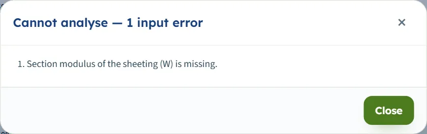
| Stop: other limits | “Width of the cut (B) must be at least 0.5 m.” · “Horizontal strut spacing (s) must be at least 0.5 m.” · “Wall embedment below the base (d) must be at least 0 m.” · “Yield strength (fy) must be at least 100000 kPa.” · “Thickness (Hi,1) must be at least 0.1 m.” · “Section modulus of the sheeting (W) is missing.” |
Where a limit applies, the window opens with Cannot analyse — 1 input error (2, 3 … when several); a condition of the solution opens Cannot analyse — a condition of the solution is not met, which ends “Nothing was calculated. Change the inputs marked in red, then press Analyze again.”
Warnings
A warning marks a result that is calculated but fails a check; the bar reads Analysed — the braced cut calculated — 1 warning and the window opens at once.
- A member fails: “The sheeting given does not carry the design moment: MEd / Mc,Rd = 1.49 …” with the resistance, the demand and the modulus the sheeting asks for (223.63 cm³/m); the wale and the strut have their own messages. The wale message suggests closing the spacing s.
- Piping: “Factor of safety against piping FS = 1.14 is below the required 1.50. The upward seepage at the base is close to lifting the sand …” with the remedies: drive the sheeting deeper, lower the head, or add a filter blanket.
- Hydrostatic pressure left out: “Water table at z = 3.00 m is above the base and the hydrostatic pressure is left out …”
- Head loss different from the wall load: “Hydraulic boundary mismatch: the piping check uses h = 2.00 m, the wall was loaded with the full head 5.00 m …” and the factor of safety is then shown with the word NOT COMPARED. Clear the head-loss box to take the head from the water table.
Notes
The default run carries five notes: that no piping check is needed with the water below the base (re-check if dewatering lowers the water inside the cut below the outside groundwater); the sheeting modulus taken as that of the whole wall; the wale checked on its modulus without shear; the strut class not computed for a strut given by A and I; and the factor γF applied before the code check.
Good practice and common mistakes
- Enter the saturated unit weight of every layer when there is a water table; the module stops if it is not above 9.81 kN/m³.
- Leave the head loss to follow the water table unless you have a flow net for another seepage picture; a different head gives a factor of safety without a verdict.
- Keep struts inside the cut and apart; drag them before Analyze, not after.
- The surcharge is not multiplied by 0.65: it acts as Ka q beside the envelope.
- Read the strut load per strut and the moment per metre of wall; the wale moment is for one span.
- Choose the hinge convention knowingly: every strut lowers the load of A and raises that of B in the example.
- Give the sheeting modulus of the whole wall from the maker’s table and take interlocks and shear from the maker’s data.
- Name the code once: the factors of EN 1993-1-1 and of AISC are different inputs.
- Keep the model: the page opens on the default every time; use Save to file… or Quick Save…, and the report as the record.
Frequently asked questions
What is the apparent pressure envelope?
A single uniform pressure over the full depth of the cut, σa = 0.65 Ka σ′v(H), taken from measured strut loads rather than from a Rankine triangle. For the example it is 28.12 kPa.
How are the strut loads found?
The sheeting is cut into pieces at its hinges and each piece is a determinate beam on the struts it holds; the reaction per metre times the spacing s is the strut load. The example gives 318.75, 175.53 and 180.60 kN.
How many struts can I use?
From 2 to 15 levels. Use the buttons Add a strut level and Remove the last strut, then type or drag the depths.
What does the hinge convention change?
Which struts the sheeting is hinged at. Auto and Interior struts hinge every strut except the top and bottom; Every strut hinges all of them. In the example the largest load falls from 318.8 to 270.0 kN with Every strut.
How is water handled?
With the water table above the base the overburden is effective, the hydrostatic pressure is added to the wall, and the piping check is made on the exit gradient. Below the base the water has no effect.
How is the piping factor of safety found?
FS = icr / iexit, with iexit = h / (Nd a) for a flow net. With h = 5 m, 8 drops, a = 1 m and icr = 1 it is 1.600, which passes the required 1.5.
Can I add a strip or point surcharge?
The Surcharge section takes a uniform load; Strip and Point are shown marked Soon.
Which members does the module verify?
The sheeting and the wale in bending, and the strut in flexural buckling, to EN 1993-1-1 or AISC 360-22 (LRFD or ASD). The wale and strut can be given from a catalogue of steel sections.
Can I drag things on the drawing?
Before Analyze you can drag the strut levels; the field follows. After Analyze there are no handles; press Edit inputs.
Does the module remember my inputs?
No: it opens on the default example every time; only the unit system is remembered. Save to file keeps the model and Quick Save keeps versions in the browser.
Which units does it use?
SI · kN, SI · tf or US, switchable at any time. The default example gives Pmax = 318.8 kN, 32.52 tf or 71.65 kip.
What if a member fails?
It reads FAIL, appears red on the drawing and a warning gives the modulus it asks for. Choose a heavier section or a higher grade, close the spacing, or add a strut level.