
On this page · 14 chapters
- 1A pile under lateral load
- 2The pile as a beam on springs
- 3The elastic solutions
- 4The p–y curve of a sand
- 5The p–y curve of a clay
- 6Layers and water
- 7The numerical solution
- 8The axial load
- 9The head and the free length
- 10Reading the results
- 11The load–deflection curve and the allowable values
- 12A worked example
- 13What the module assumes
- 14References
A pile pushed sideways bends over its upper length and is held by the ground along it. This page explains, section by section, how the module finds how far the head moves and how large the moment and the shear in the pile get: the pile as a beam on springs, the elastic solutions, the p–y curves of sand and clay, the layers and the water, the numerical solution, the axial load, the head, the load–deflection curve, a worked example whose every number is computed by the module’s own engine, and the assumptions.
 PDF
Lecture slides
Ready-made slides for lectures and self-study
The mechanism, the derivation, the equations and the figures of this page, in teaching order. Every slide links back to its chapter.
1A pile under lateral loadwhat happens, and the methods of analysis
A pile that carries a lateral load — wind, a braking force, a mooring pull, an earthquake acting on the structure, the thrust of a retained soil — does not fail the way a footing does. The load reaches the ground only through the sideways movement of the pile, and the ground answers with a reaction that grows with that movement and stops growing when the soil yields. The pile bends, like a beam, over the first few diameters below the ground; deeper than that the ground is hardly moved and the pile is straight. How much it deflects and how large the bending moment gets depend on the stiffness of the pile, on the stiffness and the strength of the ground at each depth, and on how the head is held.
Three families of methods are in use, and the source treats all three:
- The ultimate load (Broms): the load at which the soil fails around a short pile, or the pile yields in bending when it is long. It gives a capacity, not the deflection or the moment at the working load.
- The elastic subgrade reaction (Matlock and Reese; Davisson and Gill; Hetényi): the ground is a row of elastic springs and the beam equation is solved in closed form. It gives the deflection and the moment of a pile whose ground stays elastic.
- The p–y method (Matlock, Reese and others): the springs are non-linear. The reaction of the ground at each depth follows a curve against the deflection — p against y — that starts stiff, softens and ends on the ultimate resistance of the soil at that depth. The equation is solved numerically. The ground can be in layers, and the answer holds from the working load to the neighbourhood of failure.
The module is the third method, and carries the second as an option: a single pile, in up to eight layers of sand or clay, with the head free or held against rotation, a free length above the ground, an axial load, and static or cyclic loading. The elastic option is there for checking the module against closed-form solutions (Section 3) and for the engineer who works with a coefficient of subgrade reaction.
2The pile as a beam on springsthe equation, the signs and the conditions at the ends
The pile is a beam. The ground is a row of springs along it, each acting on its own depth and independent of the others — the Winkler model. With z down from the ground surface and y the deflection of the pile in the direction of the load, the equation of the beam is
The reaction p is positive when it opposes the deflection. For a spring of stiffness k, p = k y. The source writes the same thing as k = p′/x: the k of the elastic solution has the unit of a force per unit length per unit deflection, kN/m². The coefficient of horizontal subgrade reaction kh of a foundation engineer is the same quantity per unit width of the pile, k = kh D.
The bending moment, the slope and the shear force follow from the deflection:
With these signs a lateral load H at the head gives V = H and a positive moment below it, as in the source. A moment Mg at the head is positive when it adds to the deflection the load causes.
The conditions at the ends
- The tip is free: M = 0 and V = 0. The pile has no base shear or base moment from the ground below its tip.
- The head carries the load H and, when it is free to rotate, the moment Mg; when it is held against rotation by a cap the slope is zero there and the moment that holds it is part of the solution.
What the equation needs, then, is the law p(y, z) of the ground: constant k times y in the elastic case, or the p–y curves of Sections 4 and 5.
3The elastic solutionsthe closed forms for sand and for clay, and the coefficients the module computes
When the ground is elastic the equation has closed-form solutions, and the source gives them.
The reaction grows with depth: sand (Matlock and Reese)
For a granular soil the coefficient of subgrade reaction is taken to grow in proportion to depth, k = nh z, nh the constant of horizontal subgrade reaction (the source gives representative values of it). The pile has one characteristic length
and its deflection, slope, moment and shear are, for a load Q and a moment Mg at the ground surface,
| Ay | Aθ | Am | By | Bθ | Bm | |
|---|---|---|---|---|---|---|
| Z = 0 | 2.429 | −1.619 | 0.000 | 1.619 | −1.747 | 1.000 |
| Z = 0.5 | 1.640 | −1.500 | 0.458 | 0.871 | −1.250 | 0.974 |
| Z = 1 | 0.961 | −1.194 | 0.725 | 0.364 | −0.789 | 0.851 |
| Z = 1.4 | 0.543 | −0.891 | 0.770 | 0.112 | −0.480 | 0.686 |
| Z = 2 | 0.142 | −0.462 | 0.627 | −0.070 | −0.153 | 0.404 |
| Z = 3 | −0.075 | −0.039 | 0.224 | −0.089 | 0.057 | 0.059 |
A worked case of the elastic solution: an HP 250 × 85 pile 25 m long in a granular soil with nh = 12 000 kN/m³, E I = 25 461 kN·m², Mg = 0. With T = 1.16 m the pile is long (L/T = 21.5). For a head deflection of 8 mm the load is Q = 8 mm × EI / (Ay T³) = 0.008 × 25 461 / (2.4292 × 1.1624³) = 53.4 kN, and the largest moment is Am T Q = 0.772 × 1.1624 × 53.4 = 47.9 kN·m; the module, at that load, gives a head deflection of 8.00 mm and a largest moment of 47.9 kN·m.
The reaction is constant with depth: clay (Davisson and Gill, Hetényi)
In a cohesive soil the coefficient of subgrade reaction is taken as constant with depth. With k the stiffness of the ground per unit length of pile, the characteristic length is R = (EI/k)1/4. The closed forms of a long pile are the ones of Hetényi for a beam on an elastic foundation; with β = (k/4EI)1/4 and a lateral load H at the ground:
The module reproduces these, and the same elastic option lets a sand layer take k = nh z and a clay layer k = kh D, in any order, which is the layered version of the two solutions.
4The p–y curve of a sandAPI RP 2A, after Reese, Cox and Koop
For a sand the module takes the p–y curve of the American Petroleum Institute (API RP 2A, 21st ed.), which Reese, Cox and Koop (1974) built from tests on a pile in sand and from the two ways the soil can fail around it. Near the ground a wedge of soil is pushed up in front of the pile; deeper the soil flows around it horizontally. The ultimate resistance at the depth z, with σ′ the effective vertical stress there, is the smaller of
and the coefficients depend on the friction angle alone:
The curve itself is the API form
At small deflection the curve is the straight line p = k z y — the elastic solution of Section 3 with nh = k, which the module reproduces to six digits at a vanishing load — and at large deflection it ends on A pu. The factor A is 3.0 at the surface and falls to 0.9 at a depth of 2.6 diameters, where it stays; it is the greater static resistance of the ground near the surface. For cyclic loading it is 0.9 at every depth.
| φ′ | C1 | C2 | C3 | k above the water table (MN/m³) | k below it (MN/m³) |
|---|---|---|---|---|---|
| 28° | 1.60 | 2.41 | 22.5 | 5.4 | 5.4 |
| 30° | 1.91 | 2.67 | 28.7 | 10.5 | 7.9 |
| 32° | 2.28 | 2.95 | 36.8 | 20.7 | 11.9 |
| 34° | 2.72 | 3.25 | 47.3 | 32.7 | 17.6 |
| 36° | 3.24 | 3.59 | 61.2 | 46.3 | 24.8 |
| 38° | 3.87 | 3.97 | 79.6 | 61.7 | 33.6 |
| 40° | 4.62 | 4.38 | 104.1 | 78.9 | 44.0 |
The effective stress σ′ is that of the layers and the water as entered (Section 6), so a sand layer under a clay, or under the water table, has the ultimate resistance its own overburden gives.
5The p–y curve of a clayMatlock’s soft-clay curve, static and cyclic
For a clay the module takes the soft-clay curve of Matlock (1970), as API RP 2A states it. The ultimate resistance at the depth z, with cu the undrained shear strength, is again the smaller of a near-surface and a deep value: a wedge failure above, the soil flowing round the pile below,
and the curve is a cube root up to a deflection of 8 y50, where y50 = 2.5 ε50 D is the deflection that carries half the ultimate resistance and ε50 the strain at half the maximum deviator stress in the undrained test:
The cube root has an infinite slope at the origin. A programme cannot use that, and the module replaces the curve below y = 0.001 y50 by a straight line from the origin to the curve (a stiffness of 50 pu/y50); the change is in deflections of a few micrometres.
Cyclic loading
Repeated loading softens a clay near the surface, where it can gap behind the pile. API reduces the curve beyond 3 y50, where the cube root has reached 0.72 pu: the resistance stays at 0.72 pu below the transition depth zR, and above it falls linearly with y, from 0.72 pu at 3 y50 to 0.72 pu z/zR at 15 y50 and beyond.
| cu | ε50 | J |
|---|---|---|
| 15 kPa | 0.020 | 0.50 |
| 30 kPa | 0.020 | 0.50 |
| 60 kPa | 0.010 | 0.25 |
| 120 kPa | 0.005 | 0.25 |
| 250 kPa | 0.005 | 0.25 |
6Layers and waterhow the ground is described along the pile
The ground is a stack of up to eight layers, each a sand or a clay, with its own unit weights and strength, and a water table at any depth. Every p–y curve is evaluated at the depth it belongs to, from the soil of that depth:
- The effective vertical stress σ′ at the depth z is the sum of the unit weights over the layers above, γ above the water table and γsat − γw below it, with γw = 9.81 kN/m³. It is not an average over the layer; the ultimate resistance of a layer grows through it with the stress.
- The layer at z gives φ′ and k (sand) or cu, ε50 and J (clay). The initial modulus k of a sand is the one for the water the layer is in; for a layer the water table crosses, it is filled in for the layer’s mid-depth, and can be typed over.
- The elements never straddle a layer boundary: there is a node at every boundary, so the stiffness of the ground jumps from one element to the next and not inside one. Where a clay lies on a sand the ultimate resistance and the stiffness change at once, and so do the diagrams.
The Calculations tab gives, for every layer, the numbers of its curve at the middle of the layer, step by step: σ′, the coefficients, pu, the factor A or y50. They are the ones the engine uses at that depth, and an engineer can reproduce them by hand; at other depths the curve is the same formula with z and σ′ of that depth. The p–y view of the module draws the curves at five depths of the part of the pile that moves.
The ground below the deepest layer entered is not described; the layers must reach the pile tip, and the pile tip is free, with no resistance from the ground below it. A pile in a ground whose stiffness is very different above and below a boundary — a soft clay over a dense sand, say — shows it in the diagrams as a kink at the boundary.
7The numerical solutionfinite elements, Newton’s method, and when there is no equilibrium
The equation of Section 2 is solved by finite elements. The pile is divided into cubic beam elements with two degrees of freedom at each node, the deflection y and the slope θ = dy/dz. The bending stiffness of an element is the one of a beam; the axial load adds the geometric stiffness of the element (Section 8). The reaction of the ground in an element is integrated at four Gauss points, where the deflection is read from the shape functions and p taken from the curve of the layer — a non-linear force of the nodal deflections, not a spring lumped at the node.
With u the nodal deflections and slopes, K the stiffness of the pile, f(u) the force of the ground and F the load, the equation to solve is K u + f(u) = F. It is solved by Newton’s method, with the stiffness of the ground at each point taken as dp/dy of the curve there:
- The slope dp/dy is not allowed to fall below a twentieth of the secant stiffness p/y: where a curve is flat or falling (the end of a clay curve, the cyclic softening) that is what is used, so that the matrix stays positive.
- A line search halves the step when it does not reduce the out-of-balance force; if even that fails, a damped step of the secant iteration, which cannot fail while the curves rise, is taken instead.
- The first estimate is the solution at a trial deflection of every spring (a fifth of y50 in a clay, one per cent of the width in a sand).
When there is no solution
If the load is more than the ground can resist, the deflection grows without limit and the iteration finds no equilibrium; the module then says so and gives no result, because a number from an iteration that did not converge would be nothing. A solution in which the ground, below the surface, has moved more than five pile widths is counted as no solution either: the p–y curves are derived for deflections of a few per cent of the width, and a ground that has moved five has failed. The same happens when the axial load reaches the buckling load of the pile in the ground (Section 8); the module calls it buckling only when the axial load alone is enough. A pile that fails under a lateral load with its axial load at work is overloaded, and is called so. The load–deflection view shows where the curve of the analysis ends.
The path to the load
With the cyclic clay curve — whose resistance falls between three and fifteen y50 above the depth zR — or with an axial load, the response of the pile is not one rising curve of load against deflection. It rises to a limit load and, past it, the same load can have a second equilibrium far from the first, soft and remote, which the pile could never reach from rest. One solution at a load beyond the limit load can land on that remote state and report it as a result. For these piles the module therefore reaches the load of the analysis in steps from no load, each solved from the one before and each refused if it throws the pile to a deflection much beyond the last; where the steps end is the limit load, and the sheet names it (the pile and the ground carry the load up to about …). Where every curve rises and there is no axial load — a static analysis, and the elastic analysis — the equilibrium is unique and one solution is enough; if that fails, the same steps find the load up to which the pile is carried.
The mesh, and the checks
The element length is a sixth of the pile width, not under 3 cm and not over 15 cm (and never less than 1/1500 of the length of the pile), with a node at every layer boundary. The largest moment and the other extremes are not read from the nodes: M has the slope V − Pθ, so the peak is where that passes through zero and its value is the cubic through the two nodes. The result does not depend on the mesh to the figures shown:
| Element length (m) | Nodes | Iterations | Head deflection (mm) | Largest moment (kN·m) | At z (m) |
|---|---|---|---|---|---|
| 0.400 | 37 | 7 | 6.228 | 151.77 | 2.14 |
| 0.200 | 71 | 7 | 6.227 | 151.77 | 2.13 |
| 0.100 | 141 | 7 | 6.228 | 151.77 | 2.13 |
| 0.050 | 281 | 7 | 6.227 | 151.77 | 2.13 |
| 0.025 | 561 | 6 | 6.228 | 151.77 | 2.13 |
Two checks are written on the Calculations tab for every run: the sum of the soil reaction over the length against the load H, which holds exactly for the solution, and the moment at the tip found by statics from the load, the ground’s reaction and the axial load, which is zero if the solution is in equilibrium. Neither depends on the finite element solution being accurate, so they check the iteration and the bookkeeping, not the model; the accuracy of the model is checked against the closed forms of Section 3 and against independent solutions of the non-linear problem — a rigid pile in clay, whose two unknowns can be solved by hand, and the elastic limit of the non-linear sand curve, to which the module reduces at a vanishing load.
An independent implementation
The whole problem has also been solved by a second program, written from the equations of this section and the two p–y curves alone, by finite differences and in another language, without sight of the module: an independent implementation written from the equations and the two p–y curves alone, by finite differences — 14 piles, static and cyclic, in sand, clay and layered ground, free and held heads, with an axial load, with a free length, with a p-multiplier, from a small to a strongly non-linear load — agrees in the head deflection and in the largest moment to within 0.01 %. The cases cover the head free and held, a moment at the head, an axial load, a free length above the ground, a water table, a p-multiplier and a pile of steel in three layers. Eight further loads of the same piles, five of them taking the cyclic curve of a clay beyond 3 y50 into its softening branch (up to 32 y50) and one the static curve beyond its plateau, agree to within 0.02 %. Where the load on the head passes a maximum before the load asked for is reached (two loads on a pile in stiff clay), the module gives that limit load — 819 and 437 kN, against 822 and 438 kN found by the second program, which imposes the deflection — and not the equilibrium beyond it, at a deflection of 0.4 and 0.55 of the pile width. That shows that the module solves the equations it states.
8The axial loadP–δ, and when the pile buckles
The axial load P acts through the deflected shape of the pile. It is in the equation (the term P d²y/dz², Section 2) and in the stiffness of every element as the geometric stiffness, which lowers the lateral stiffness of a compressed beam and raises the deflection and the moment. The module takes P as constant over the whole length of the pile and the same at the head and the tip. In reality the skin friction passes part of the load to the ground, so the load at depth is less; taking it constant is on the safe side.
A compressed pile in an elastic ground has a buckling load. For a pile long enough that its tip does not move, in ground of constant stiffness k per unit length, the closed form of the semi-infinite beam shows that a free head loses its stability at P = √(k EI) — half of the 2√(k EI) of an infinite beam, because the free end can rotate. The load–deflection of such a pile rises without limit as P approaches it, and the module, whose stiffness matrix then stops being positive, says that the axial load exceeds the buckling load in this ground. A head held against rotation buckles at a higher load. The module checks the pile as a beam on springs; the strength of the pile section under the axial load and the moment together is a check of the structural design.
9The head and the free lengthfree, held, and a load above the ground
Three arrangements of the head are in the module.
- Free head. V = H and M = Mg at the point of the load.
- Held head. The slope is zero and the head moves sideways. A pile in a long, uniform, elastic ground deflects half as much as the free one (Section 3), and the moment that holds the head, M = −H/(2β) there, is larger than the largest moment of the free pile in such a ground; the module gives it as the moment at the head and marks it in the diagrams. How near a real cap comes to this depends on the stiffness of the cap and the superstructure, and the real condition lies between the two.
- A free length e above the ground. The pile above the ground has no ground to act on it and bends as a cantilever. The shear is H all the way down to the ground and the moment grows to M(0) = Mg + H e at the ground surface, where the ground takes over. The deflection of the head is the deflection of the pile at the ground plus the rotation there times e plus the cantilever deflection of the free length: a given load with a free length gives a much larger deflection of the head than of the ground, and the largest moment is usually at the ground or a little below it.
10Reading the resultswhat each result is, and the diagrams
The Results tab gives the response at the load entered; the Diagrams tab draws it along the pile.
- The deflection of the head y at the point of the load, and at the ground surface when there is a free length, with the rotation there (the slope dy/dz, negative for a pile that leans over in the direction of the load).
- The largest bending moment and its depth. With a held head the head moment is listed too, since it is not always the largest.
- The depth of zero deflection, where the pile crosses its own axis: the pile moves into the ground above it and away from it below.
- The shear and the soil reaction along the pile, the reaction with the end of the p–y curve drawn beside it, so that one can see where the ground is near its limit.
- The tip. A pile that is long enough has no deflection at the tip. When the tip moves, the pile is short for this load in this ground; it turns as a rigid body about a point near its lower end, and its length governs the result. The module says so when the tip moves by more than a tenth of the deflection at the ground and by more than 2 mm.
The p–y view draws the curves of the ground at five depths over the part of the pile that moves, with the point each has reached marked on it. A point on the straight beginning of a curve is a depth where the ground is working elastically; one near the end is at its limit.
11The load–deflection curve and the allowable valuesthe load at an allowable deflection or at the moment capacity
Because the ground is non-linear, the deflection is not proportional to the load, and the load at an allowable deflection cannot be read from the one at the working load. The module raises the load and the moment at the head in proportion — a factor λ on H and Mg, the axial load kept — solves the equation again at each, and finds the λ at which the head deflection reaches the allowable value, or the largest moment the capacity of the section. The result is the load Hy or HM on the Results tab.
When the ground cannot carry the allowable value — there is no equilibrium before it is reached — the module says not reached and the curve ends at a cross at the largest load it did solve. For a pile whose response folds (the cyclic clay curve, an axial load) it is the limit load of the ground. It is not a capacity of the pile: the pile is elastic in the module, and a pile that yields in bending may fail before the ground does. The moment capacity entered is the check of that. The module gives no factor of safety and takes none from a code; the allowable deflection and the moment capacity are the engineer’s.
12A worked exampleevery number computed by the module’s own code
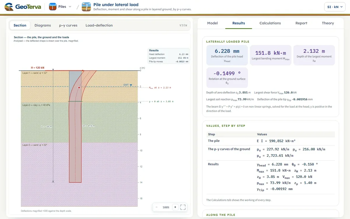
The model the Model tab opens with: a pile of 0.6 m diameter and 14 m length, in concrete (E = 30 000 MPa, E I = 190 852 kN·m²), in a ground of sand (4 m, φ′ = 32°), clay (5 m, cu = 40 kPa) and sand (8 m, φ′ = 32°), with the water table 2 m below the ground; a lateral load of 120 kN at the ground surface, the head free, static loading. Every number below is computed by the module’s own engine as this page opens.
The curves of the layers at their middle
- Layer-1, sand φ′ = 32°, at z = 2.00 m: σ′ = 36.0 kPa, pu = 227.9 kN/m, k = 20.7 MN/m³
- Layer-2, clay cu = 40 kPa, at z = 6.50 m: σ′ = 77.4 kPa, pu = 216.0 kN/m, y50 = 30.0 mm
- Layer-3, sand φ′ = 32°, at z = 11.50 m: σ′ = 123.3 kPa, pu = 2723.6 kN/m, k = 11.9 MN/m³
The response
The head deflects 6.23 mm and rotates 0.150°. The largest bending moment is 151.8 kN·m at 2.13 m below the ground, in the sand of Layer-1; the pile crosses its axis at 3.85 m, in the sand of Layer-1, and the tip moves 0.0019 mm — the pile is long for this load. The largest soil reaction is 74.0 kN/m at 1.40 m; the curve of the ground there ends on 142 kN/m, so the ground works at about 52 % of its limit.
The checks of the sheet: Σ p Δz = 120.000 kN against H = 120 kN; the moment at the tip by statics 0.000 kN·m; 7 Newton iterations.
The same pile with other choices
| Case | Head deflection (mm) | Largest moment (kN·m) | At z (m) | Zero deflection at (m) |
|---|---|---|---|---|
| As entered: head free, load at the ground, static | 6.23 | 152 | 2.13 | 3.85 |
| Head held against rotation | 2.24 | −175 | 0.00 | 4.94 |
| Load 1.5 m above the ground (free length e = 1.5 m) | 20.23 | 306 | 1.68 | 3.37 |
| Cyclic loading (API cyclic curves) | 7.28 | 172 | 2.22 | 3.89 |
| Axial load P = 800 kN (P–δ) | 6.32 | 155 | 2.13 | 3.83 |
| Cracked section, E I × 0.6 | 7.93 | 140 | 1.95 | 3.45 |
| Elastic subgrade reaction (nh = 8 MN/m³ in sand, kh = 15 MN/m³ in clay) | 10.49 | 173 | 2.49 | 4.10 |
Held against rotation, the head deflects 2.24 mm instead of 6.23 mm, and a hogging moment of 175 kN·m acts at the head, 15 % above the largest moment of the free pile. With the load 1.5 m above the ground the head deflects 20.2 mm (11.1 mm at the ground) and the largest moment is 306 kN·m. Cyclic loading raises the deflection by 17 %: the sand near the surface loses the factor A of the static curve. An axial load of 800 kN raises it by 2 %; a section cracked to 0.6 E I by 27 %, with a smaller largest moment (140 kN·m) because the pile is more flexible. The elastic ground, with the nh and kh the Model tab fills in, gives 10.5 mm; its constants are the engineer’s, so it is another ground and not a check of the p–y curves.
13What the module assumesthe assumptions behind the numbers, in one place
Every analysis rests on assumptions. The module sorts them by how they reach the results:
- One pile. A single pile, with no neighbour, on the p–y curves of a pile standing alone. A group of piles loaded sideways deflects more than a single pile under the same load on each pile, because the soil between the piles is shared and the rows behind the first are shadowed; the group, with the p-multipliers of its rows, is the subject of the pile group module.
- The pile. One section over the whole length, linear elastic: E I is constant along the pile and under the moment and the axial load. A concrete section that cracks is represented by the factor on E I entered with the section, and the moment at which the section yields by the capacity Mcap entered with it.
- The ground. Independent springs, no shear between them, with the curves of Sections 4 and 5. The curves are empirical, from tests in particular soils: the sand curve rests on φ′ alone, and the clay curve on cu and ε50. They describe a sand and a soft to medium clay as the pile meets them, the ground as entered around it, with the cyclic reduction of API for repeated loading; a stiff clay, a weathered rock, a cemented soil and a liquefied sand are described by curves of their own.
- The loading. Static, or cyclic by the API reduction, applied at the head: the lateral load H, together with a moment Mg when the head is free.
- The axial load is constant over the length: the load P entered at the head.
- The numerical solution is by finite elements with a non-linear iteration; it is exact to the figures shown for the equation as given; the approximation is in the equation, which represents the ground by springs.
The p–y method is the basis of the design of laterally loaded piles in practice. The curves the module carries are a good model for a pile in sand and in a soft or medium clay, and the numbers they give are to be set against the allowable values of the project, and against a load test where one is available.
14Referencesthe elastic solutions, the p–y curves and the method
- Das, B.M. (2016). Principles of Foundation Engineering, 8th ed. Cengage Learning, Boston.
- Matlock, H. and Reese, L.C. (1960). Generalized solutions for laterally loaded piles. Journal of the Soil Mechanics and Foundations Division, ASCE, 86(SM5), 63–91.
- Matlock, H. (1970). Correlations for design of laterally loaded piles in soft clay. Proceedings of the 2nd Offshore Technology Conference, Houston, Paper OTC 1204, 577–594.
- Reese, L.C., Cox, W.R. and Koop, F.D. (1974). Analysis of laterally loaded piles in sand. Proceedings of the 6th Offshore Technology Conference, Houston, Paper OTC 2080, 473–485.
- American Petroleum Institute (2000). Recommended Practice for Planning, Designing and Constructing Fixed Offshore Platforms — Working Stress Design, API RP 2A-WSD, 21st ed.
- Hetényi, M. (1946). Beams on Elastic Foundation. University of Michigan Press, Ann Arbor.
- Reese, L.C., Isenhower, W.M. and Wang, S.-T. (2006). Analysis and Design of Shallow and Deep Foundations. John Wiley & Sons, Hoboken.
- Broms, B.B. (1965). Design of laterally loaded piles. Journal of the Soil Mechanics and Foundations Division, ASCE, 91(SM3), 79–99.
- Reese, L.C. and Welch, R.C. (1975). Lateral loading of deep foundations in stiff clay. Journal of the Geotechnical Engineering Division, ASCE, 101(GT7), 633–649.
- Davisson, M.T. and Gill, H.L. (1963). Laterally loaded piles in a layered soil system. Journal of the Soil Mechanics and Foundations Division, ASCE, 89(SM3), 63–94.
From theory to your own design
Analyse your own laterally loaded pile in minutes
- Deflection, rotation, moment, shear and soil reaction along the pile
- The p–y curves at five depths, static or cyclic
- The load at an allowable deflection or moment
- A clean calculation report, saved as a PDF. Online: nothing to install, no dongle, on a phone, a tablet or a PC