

What the module calculates
Cantilever RC wall checks a reinforced-concrete cantilever retaining wall, a stem on a base slab with a toe and a heel, for sliding, overturning, eccentricity and bearing pressure, in the static case and in the seismic cases, and gives the shear force and bending moment in the stem, the toe and heel slabs, the shelf and the key. Every force is drawn and listed, so each factor of safety can be followed by hand.
The earth pressure acts on the vertical plane through the heel edge, soil against soil, so the thrust is parallel to the backfill surface. The sliding factor is:
Neff is the vertical force on the base with the uplift taken off, Hdrive the horizontal force that pushes the wall, and Ptoe and Pkey the passive resistance of the soil in front of the base and of the key, used in sliding only. Overturning is taken about the front bottom corner of the base slab (the toe edge, point O), and the eccentricity and the bearing pressure are referred to the base underside about the same point.
What you can describe
- A stem of constant or tapered thickness (the back face or the front face stays vertical), a toe, a heel and a base slab, with an optional pressure-relief shelf on the back of the stem and an optional shear key under the base.
- A flat or inclined backfill (β above −45° and below 45°), a passive-side fill over the toe, and one soil for the backfill, the front fill and the foundation.
- Uniform, strip and point surcharges (up to six loads), groundwater on the retained side and on the front side, and base uplift.
- Rankine or Coulomb static earth pressure and Mononobe–Okabe seismic earth pressure, with the hydrodynamic water pressure and the inertia of the wall and of the soil that moves with it.
Which module for which wall
- A gravity wall in stone masonry or plain concrete on a stepped footing: Gravity wall.
- A reinforced-soil wall: MSE wall.
- The pressure of a surcharge on its own, or the earth pressure of a layered or sloping ground behind a wall of your own: the modules of Surcharge loads and Lateral earth pressure.
- A bearing capacity with depth, shape and inclination factors: Bearing capacity. Here the bearing pressure under the base is compared with the allowable pressure qall that you enter.
- The family overview is on the Retaining walls page.
Before you start: what you need
Have these ready from your design and your ground investigation:
| What | Notes |
|---|---|
| The wall section From: Your design | Retained height H, stem thickness at the top and at the base, toe and heel projections, base slab thickness; a shelf or a key if you use them. |
| The soil From: Boring logs and tests | Moist and saturated unit weight, the effective friction angle φ′ (cohesion is taken as zero), the base friction coefficient μb and the allowable bearing pressure qall. |
| The backfill and the front fill From: Your design | The slope angle β of the backfill and the height hp of the soil in front of the wall above the base top. |
| Loads and water From: Your design loading, groundwater readings | Surcharges, the depth of the water table behind the wall and, if any, the water height in front of it. |
| The earthquake From: Your seismic study | The horizontal and vertical coefficients kh and kv; the module does not derive them. |
| The required factors From: Your design basis | Minimum sliding and overturning factors for the static and the seismic case. |
Quick start in seven steps
- Open the module and choose the units
Open Cantilever RC wall from the Retaining Walls family. Pick SI · kN, SI · tf or US in the header; you can change it at any time.
- Draw the wall
In Geometry type H, the stem thickness (constant or variable), the toe, the heel and the base slab. In Optional geometry switch the shelf and the key on or off and size them.
- Describe the ground
Set the backfill in Backfill Slope, the front fill in Passive-Side Fill and the soil in Soil Definition.
- Add loads, water and the earthquake
Add surcharges in Surcharge Load, the water table in Groundwater and, if needed, choose Yes in Earthquake and enter kh and kv.
- Set the criteria and the method
Check the minimum factors in Stability criteria, and the static method and the passive resistance in Analysis Settings.
- Press Analyze
Press Analyze in the bar at the foot of the Model tab. A window reports the outcome, the inputs lock, and the drawing and the four cards below it fill in.
- Read the answer
The Results tab gives the checks, the forces and the structural actions. Pressure and Forces show them on the wall; Calculations writes out the working and Report saves a PDF or a Word file.
The screen: four views and four cards
The layout is the one every GeoTerva module shares, described in the workspace guide. The drawing on the left has four views, chosen with the buttons above it:
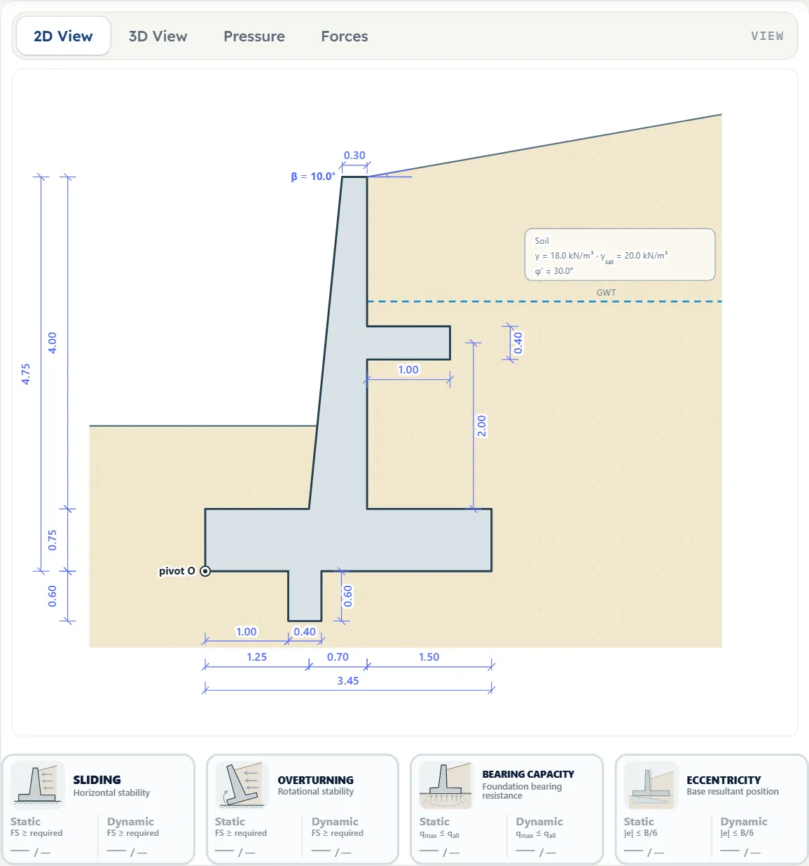
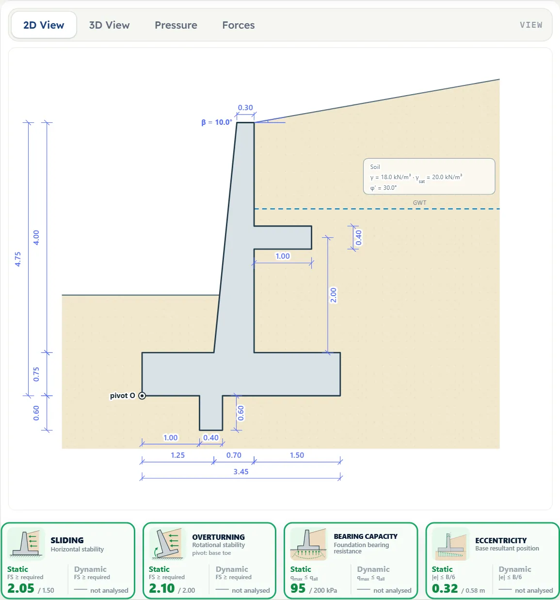
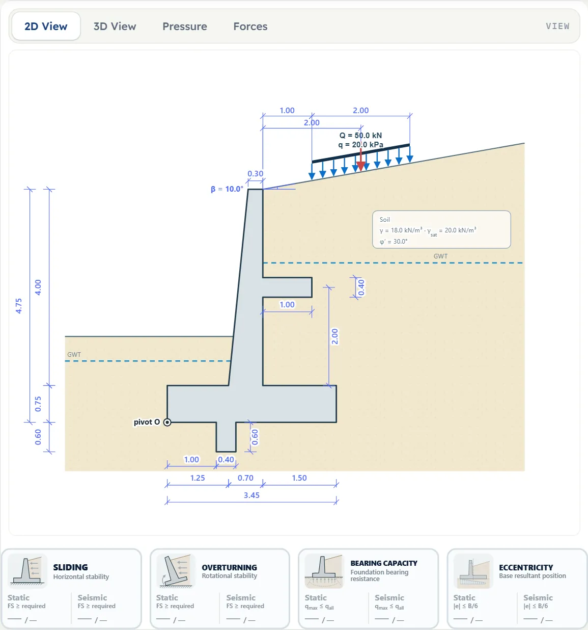
- 2D View is the section of the wall as you have modelled it, with the dimensions in the unit system you chose, the soil label, the groundwater lines, the shelf, the key, the surcharges and the ringed overturning pivot O. It changes as you type.
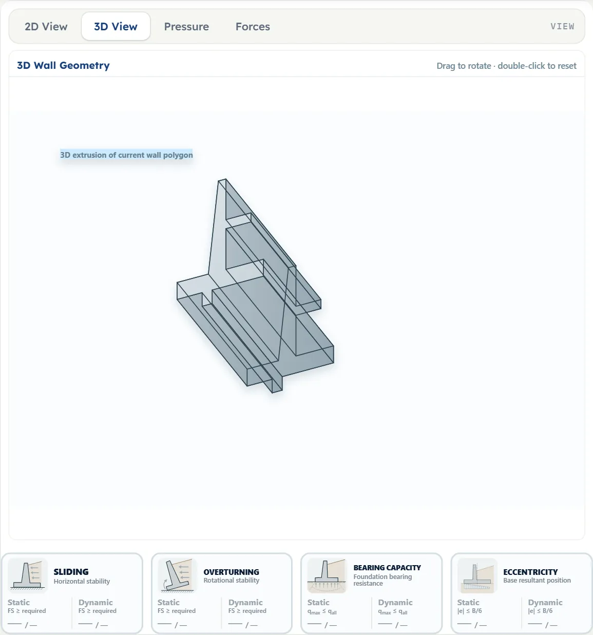
- 3D View shows the wall as a solid. Drag to rotate, double-click to reset (the hint is on the drawing).
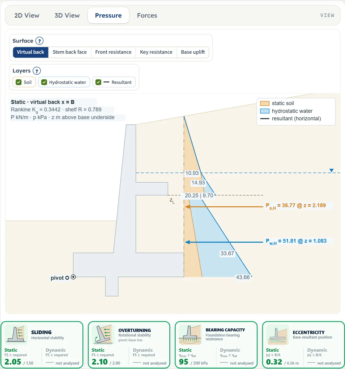
- Pressure is available after Analyze: the pressure diagrams on the wall, with the resultants and their heights.
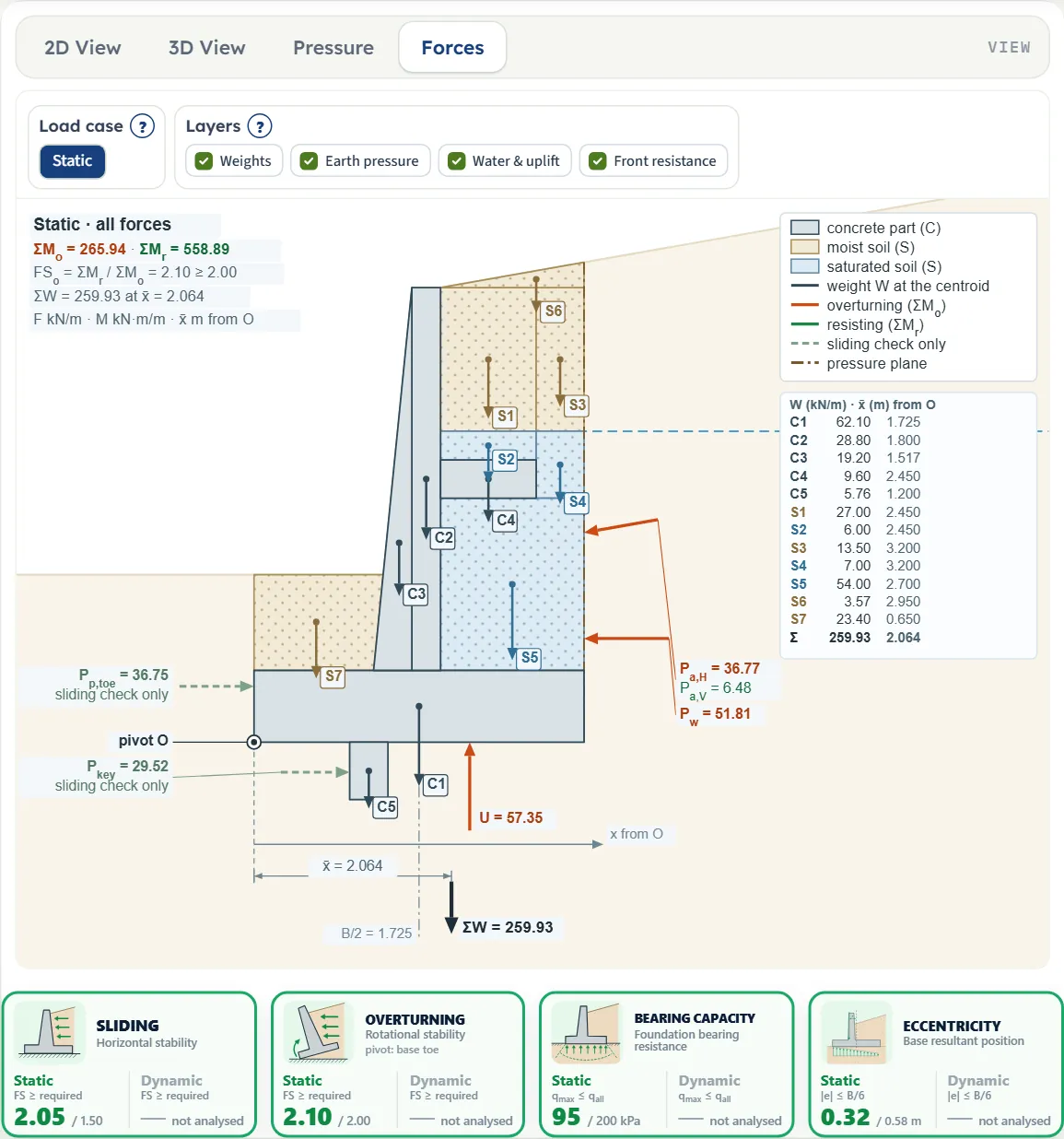
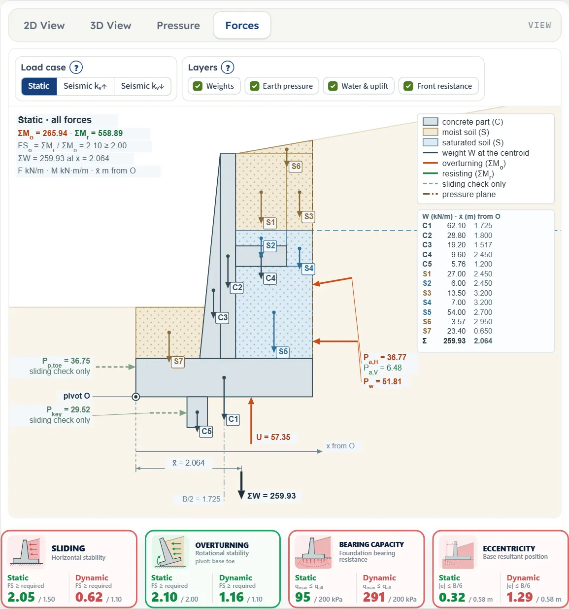
- Forces is available after Analyze: the free body of the weights, the pressures, the uplift and the passive resistances, with the lever arms from O.
The four cards
Under the drawing, Sliding, Overturning, Bearing capacity and Eccentricity each show a Static and a Seismic value with its requirement. Before Analyze they are grey; after it they turn green or red, and pressing a card opens the Results tab. Seismic reads “not analysed” until the earthquake is on. The overturning card names the pivot.

The Pressure and Forces bars
Each of these two views has a bar of its own, and it lists only what the model contains. In Pressure, Surface chooses the plane: Virtual back always, Stem back face with a shelf, Front resistance, Key resistance and Base uplift when they exist; Layers shows or hides Soil, Hydrostatic water and Resultant, with Surcharge, Strip & point loads, Seismic increment, Seismic total and Hydrodynamic water added when the model has them; with the earthquake on, Load case switches between the static case and the seismic cases. In Forces, Load case and Layers (Weights, Earth pressure, Water & uplift, Front resistance, and Surcharge and Seismic when present) do the same. The (?) beside each group says that the layers are display only: the checks always use every component.
Entering the model, section by section
The Model tab has twelve sections: Model data, Geometry, Optional geometry, Backfill Slope, Passive-Side Fill, Soil Definition, Surcharge Load, Groundwater, Earthquake, Concrete & reinforcement, Stability criteria and Analysis Settings. Model data opens and closes on its own; of the others one is open at a time, so opening one closes the previous one. Next and Back at the foot walk you through them, and Analyze waits in the bar at the bottom. Where a unit is shown twice or three times, such as m · ft, the units are those of SI · kN, SI · tf and US in turn. Defaults are shown in SI; a unit switch converts the boxes (the 4 m wall reads 13.12 ft).
Model data
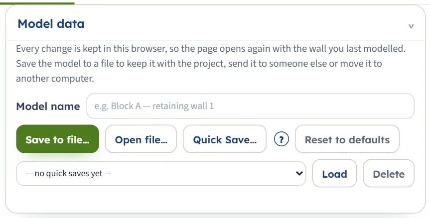
The first section holds the model name, Save to file…, Open file…, Quick Save… with its (?), the list of quick saves with Load and Delete, and Reset to defaults. A line under the buttons says what was restored when the page opened. Save to file writes a .gtrv file named after the model; Quick Save keeps a version in this browser, with its inputs, its analysed state and the report cover.
Geometry
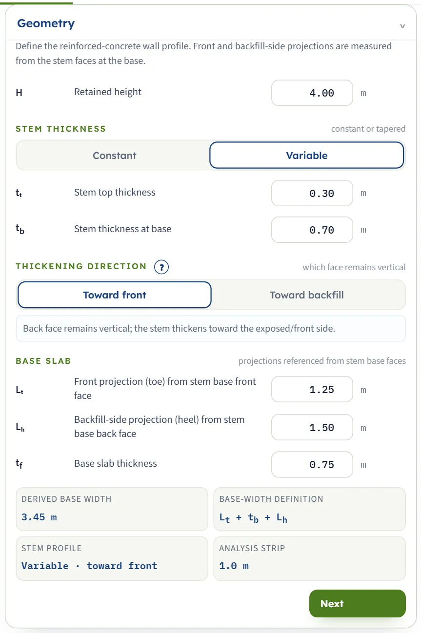
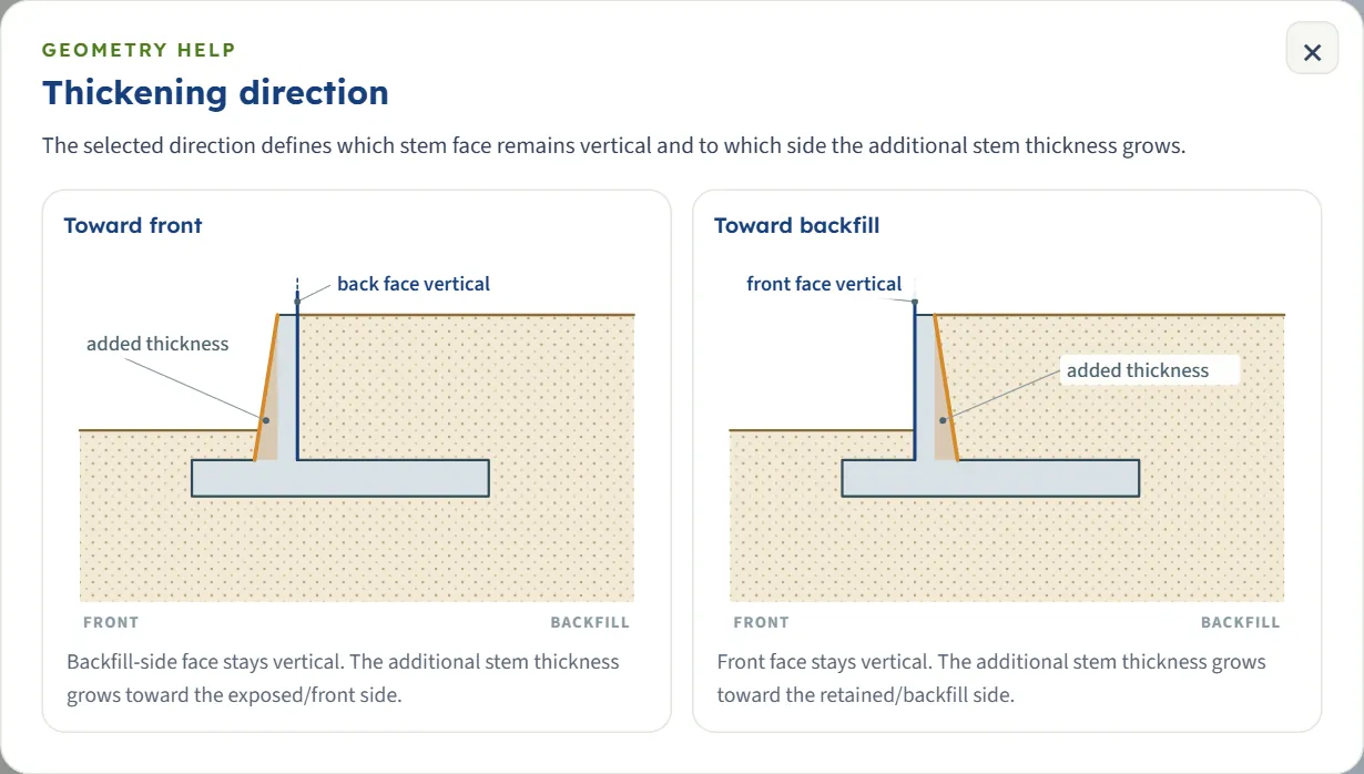
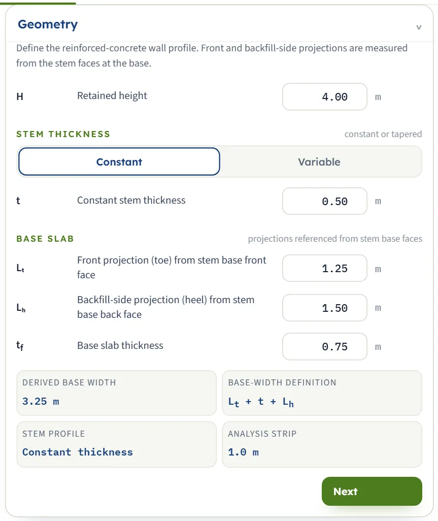
Stem thickness has Constant (one thickness t, default 0.50 m) and Variable, the default, with a top thickness tt and a base thickness tb. With Variable, Thickening direction (Toward front, the default, or Toward backfill) says which face of the stem stays vertical; the (?) opens a sketch of both. Four read-only cards give the derived base width B = Lt + tb + Lh, its definition, the stem profile and the analysis strip (1.0 m: all forces are per metre of wall).
| Field | Default | What to enter |
|---|---|---|
| Retained height H m · ft | 4.00 | From the base top to the wall top. |
| Stem top thickness tt m · ft | 0.30 | With Variable. |
| Stem thickness at base tb m · ft | 0.70 | With Variable; at least the top thickness. |
| Constant stem thickness t m · ft | 0.50 | With Constant. |
| Front projection (toe) from stem base front face Lt m · ft | 1.25 | Measured from the front face of the stem at its base. Zero or more. |
| Backfill-side projection (heel) from stem base back face Lh m · ft | 1.50 | Measured from the back face of the stem at its base. Zero or more. |
| Base slab thickness tf m · ft | 0.75 | Greater than zero. |
Optional geometry
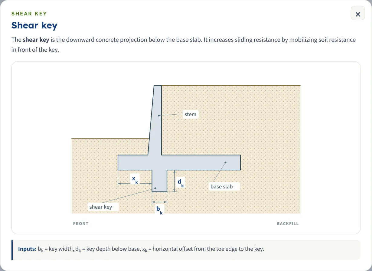
Two switches, each with an Include toggle and a (?), both on in the example. Pressure-relief shelf: a horizontal slab on the back of the stem. Below its underside the self-weight pressure of the soil restarts and is reduced by a relief ratio R = min(Ls / bkr, 1); the surcharge and the water are not reduced. Shear key: a downward projection under the base that adds passive resistance in sliding.
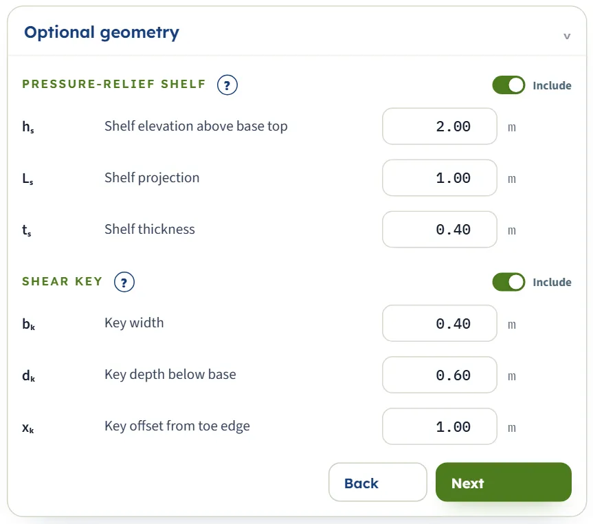
| Field | Default | What to enter |
|---|---|---|
| Shelf elevation above base top hs m · ft | 2.00 | The mid-height of the shelf. The whole shelf must lie within the stem height. |
| Shelf projection Ls m · ft | 1.00 | Greater than zero. |
| Shelf thickness ts m · ft | 0.40 | Greater than zero. |
| Key width bk m · ft | 0.40 | Greater than zero. |
| Key depth below base dk m · ft | 0.60 | Greater than zero. |
| Key offset from toe edge xk m · ft | 1.00 | From 0 to B − bk: the key must lie under the base. |
Backfill Slope
Flat or Inclined, the default. With Inclined, enter the angle β of the backfill surface, above −45° and below 45° (default 10°); a positive angle rises away from the wall. Flat sets β = 0. The uniform surcharge follows the ground line. Two read-only cards state the surface mode and the slope. The size of β must also stay smaller than φ′, for a negative angle as well (see Messages).
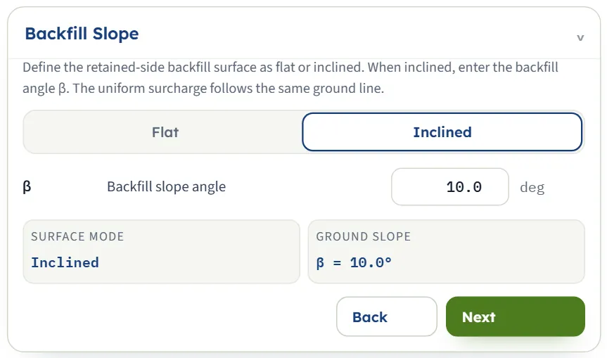
| Field | Default | What to enter |
|---|---|---|
| Backfill slope angle β deg | 10.0 | Used with Inclined. |
Passive-Side Fill
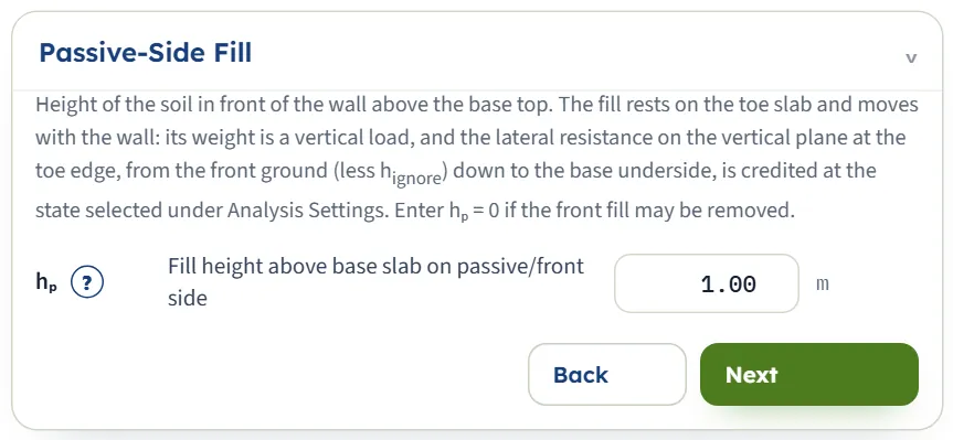
The soil in front of the wall above the base top. It rests on the toe slab and moves with the wall: its weight is a vertical load, and its lateral resistance on the vertical plane at the toe edge is credited in sliding at the passive state chosen in Analysis Settings. Enter hp = 0 if the front fill may be removed. The (?) opens a sketch of how hp is measured.
| Field | Default | What to enter |
|---|---|---|
| Fill height above base slab on passive/front side hp m · ft | 1.00 | From 0 to H. |
Soil Definition
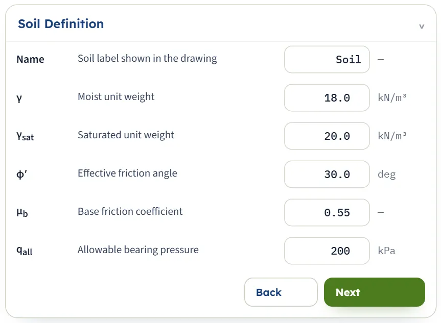
One soil serves the backfill, the front fill and the foundation. Cohesion is taken as zero. The name is only a label on the drawing.
| Field | Default | What to enter |
|---|---|---|
| Soil label shown in the drawing — | Soil | Text shown in the drawing. |
| Moist unit weight γ kN/m³ · t/m³ · pcf | 18.0 | Greater than zero. Above the water table. |
| Saturated unit weight γsat kN/m³ · t/m³ · pcf | 20.0 | Above the unit weight of water. |
| Effective friction angle φ′ deg | 30.0 | Above 0° and below 60°. |
| Base friction coefficient μb — | 0.55 | Greater than zero. Friction on the base underside: μb Neff; no adhesion is used. |
| Allowable bearing pressure qall kPa · t/m² · ksf | 200 | Greater than zero. The limit for the largest base pressure. |
Surcharge Load
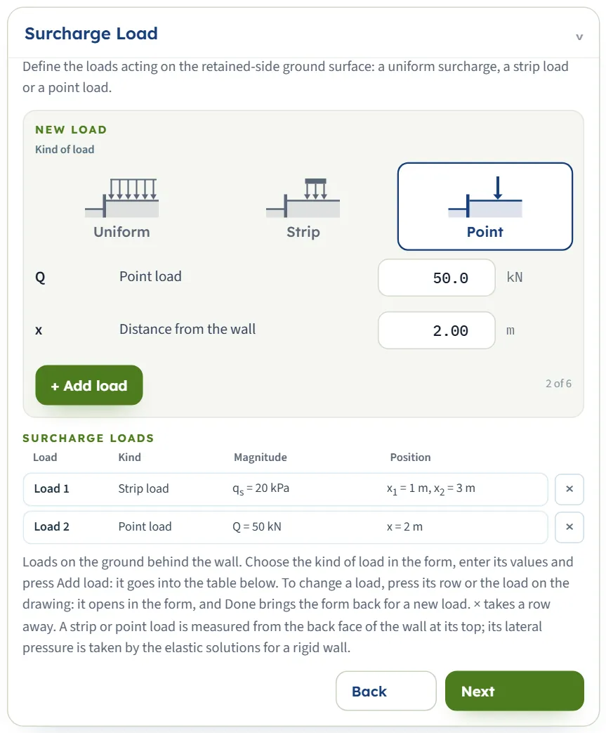
The form is the one of the sheet-pile modules. Choose the kind of load by its picture, enter its values and press + Add load: it goes into the Surcharge loads table (Load, Kind, Magnitude, Position). Press a row to edit it in the form (the form then says “Changes apply as they are entered.”, Done brings back the form for a new load and Delete load removes the load); × removes a row. Up to six loads (the form counts “2 of 6”). A strip or point load is measured from the back face of the wall at its top, and its lateral pressure is taken by the elastic solutions for a rigid wall. The uniform loads of the table add up into one uniform surcharge q. A point load closer than 0.30 m to the wall is calculated as if it stood at 0.30 m.
| Field | Default | What to enter |
|---|---|---|
| Uniform surcharge on the retained surface q kPa · t/m² · ksf | 10 | The value a new uniform load starts from. Zero or more. |
| Strip load qs kPa · t/m² · ksf | 20 | Zero or more. |
| Near edge from the wall x1 m · ft | 1 | Zero or more. |
| Far edge from the wall x2 m · ft | 3 | Greater than the near edge. |
| Point load Q kN · tf · kip | empty | Zero or more; enter it before Add load. |
| Distance from the wall x m · ft | empty | Zero or more; enter it before Add load. |
The example has no surcharge: the table is empty and the surcharge is off.
Groundwater
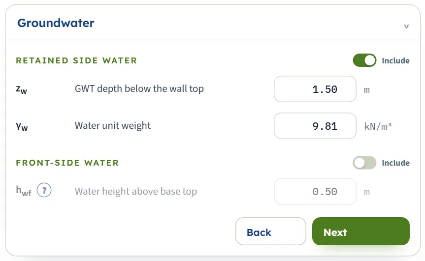
Retained side water (Include, on in the example): the water table at the depth zw below the wall top and the unit weight of water. Front-side water (off in the example): a water level in front of the wall, as a height hwf above the base top; the (?) shows how it is measured. Front water is assumed present in every load case as a favourable load.
| Field | Default | What to enter |
|---|---|---|
| GWT depth below the wall top zw m · ft | 1.50 | Zero or more. |
| Water unit weight γw kN/m³ · t/m³ · pcf | 9.81 | Below the saturated unit weight. |
| Water height above base top hwf m · ft | 0.50 | Zero or more; the box is enabled with front-side water. |
Earthquake
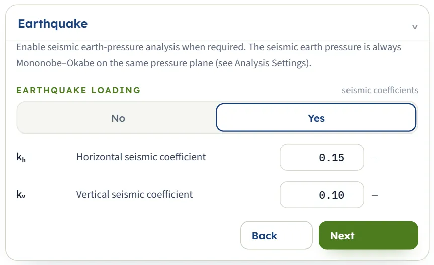
No (the default) or Yes. With Yes the two boxes open and the module adds the seismic cases. The seismic earth pressure is always Mononobe–Okabe on the same plane as the static method.
| Field | Default | What to enter |
|---|---|---|
| Horizontal seismic coefficient kh — | 0.15 | From 0 to below 1. |
| Vertical seismic coefficient kv — | 0.10 | From 0 to below 1. With kv above zero two cases are run, the vertical acceleration upward and downward; the lower factor governs. |
Concrete & reinforcement
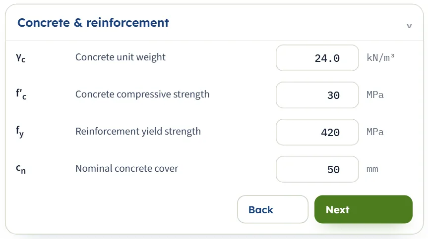
Four values. Only the concrete unit weight enters the weights of the concrete parts. The strength f′c, the yield strength fy and the cover are kept with the model and do not change any result (changing them leaves every number of the example as it was).
| Field | Default | What to enter |
|---|---|---|
| Concrete unit weight γc kN/m³ · t/m³ · pcf | 24.0 | Greater than zero. |
| Concrete compressive strength f′c MPa | 30 | Kept with the model. |
| Reinforcement yield strength fy MPa | 420 | Kept with the model. |
| Nominal concrete cover cn mm | 50 | Kept with the model. |
Stability criteria
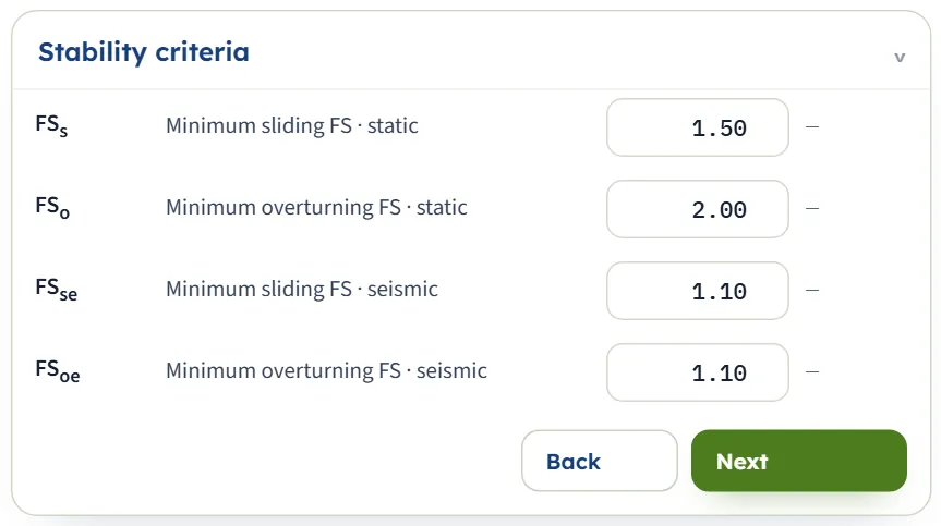
The minimum factors the checks are compared with. They appear on the cards and in the report as “required”.
| Field | Default | What to enter |
|---|---|---|
| Minimum sliding FS, static FSs — | 1.50 | Greater than zero. |
| Minimum overturning FS, static FSo — | 2.00 | Greater than zero. |
| Minimum sliding FS, seismic FSse — | 1.10 | Greater than zero. |
| Minimum overturning FS, seismic FSoe — | 1.10 | Greater than zero. |
Analysis Settings
Described in the next section: the static method, the seismic pressure, the passive resistance and the base uplift.
Choosing the method and the passive resistance
Static earth pressure is Rankine (the default) or Coulomb. Both act on the vertical plane through the heel edge, soil against soil, with the wall friction angle equal to β; for that plane the Coulomb Ka equals the Rankine Kaβ exactly, and the example gives the same answer with either (2.05, 2.10, 94.72 kPa). The Seismic earth pressure is Mononobe–Okabe, used when Earthquake is Yes; its increment acts at 0.6 h above the bottom of the plane.
Then the passive resistance, which is used in the sliding check only:
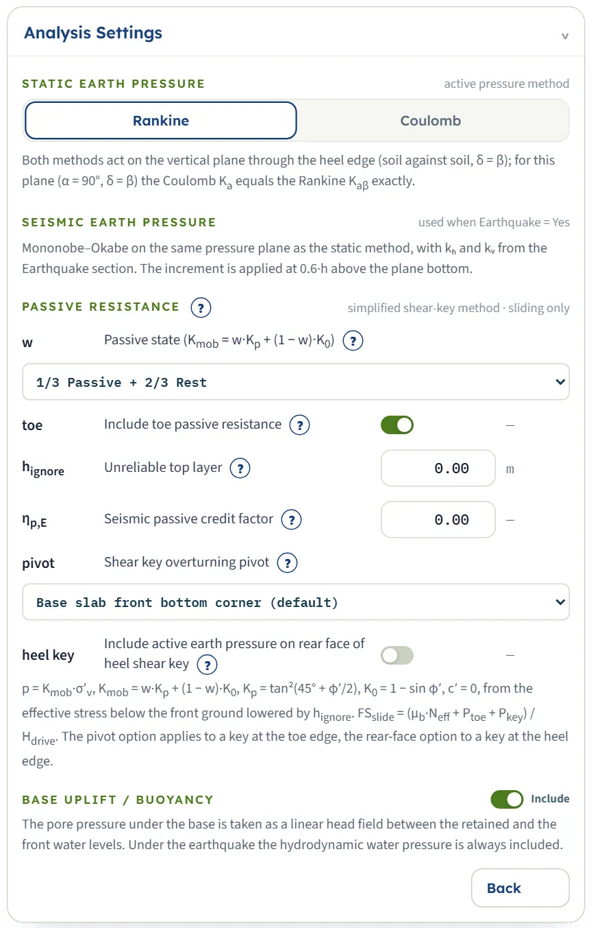
| Setting | Default | What it does |
|---|---|---|
| Passive state w Full Passive, 2/3 Passive + 1/3 Rest, 1/3 Passive + 2/3 Rest, Full Rest | 1/3 Passive + 2/3 Rest | Kmob = w Kp + (1 − w) K0, with Kp = tan²(45° + φ′/2) and K0 = 1 − sin φ′. For 30° that is Kp = 3.0000, K0 = 0.5000 and Kmob = 1.3333 in the example. The passive pressure is Kmob times the effective vertical stress. |
| Include toe passive resistance toe | On | Adds Ptoe = ∫ Kmob σ′v dz over the soil in front of the base slab. Off: the weight of the front fill still counts, its lateral resistance does not. |
| Unreliable top layer hignore | 0.00 m | The passive stresses start from the front ground lowered by this depth (frost, erosion, future trenches). |
| Seismic passive credit factor ηp,E | 0.00 | Between 0 and 1: the share of Ptoe and Pkey credited in the seismic cases. At 0 the seismic sliding rests on base friction alone. |
| Shear key overturning pivot Base slab front bottom corner (default), Shear-key front bottom corner | Base slab front bottom corner (default) | For a key at the toe edge, the choice of the shear-key front bottom corner as the pivot adds the key depth to every horizontal arm and gives a lower FSo. |
| Include active earth pressure on rear face of heel shear key | Off | For a key at the heel edge, includes the active earth pressure on the rear face of the key. |
| Base uplift / buoyancy | Include (on) | The pore pressure under the base is a linear head field between the retained and the front water levels, and reduces Neff. Under the earthquake the hydrodynamic water pressure is always included. |
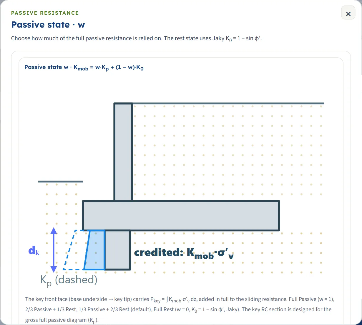
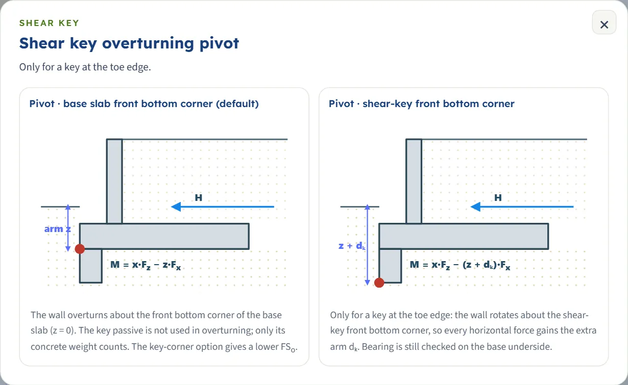
How the options change the answer
- Passive state moves FSs only: 1.58 at Full Rest, 2.05 at the default, 2.98 at Full Passive. Overturning and bearing stay at 2.10 and 94.72 kPa.
- Toe passive off gives FSs = 1.63; hignore = 0.5 m gives 1.76.
- A shelf and a key both help sliding; see the table of what-ifs below.
Analyze and read the results
Press Analyze. A progress bar steps through reading the model, earth pressure and stability, the detailed sheet, the summary sheet, the results and the report; then a window states the outcome and the bar at the foot reads Analysed — all checks satisfied or Analysed — N warnings, with the message “The inputs and the analysis settings are locked. Edit inputs clears the results; the unit system can still be changed.” Edit inputs asks “The results will be cleared. Edit the inputs?” and then unlocks the model. The module stays on the Model tab, so press Results to see the numbers.


When the run carries warnings the window is titled Attention — N warnings, says “Review these points before the results are used.” and lists each one with the reason and what to do; Show results and Stay on the model follow. A Warnings (N) button in the bar and in the tabs reopens the list. The warnings are the module’s own cautions, listed in Messages below.
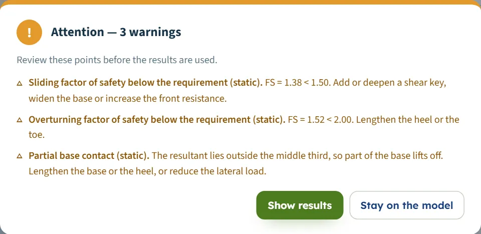
The Results tab
Blocks from the top:
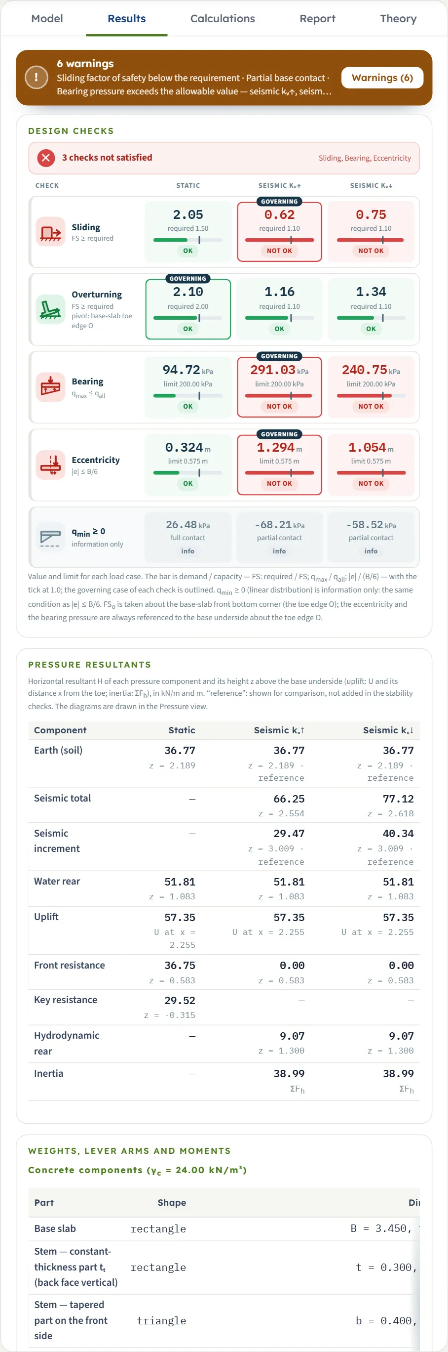
- Design checks: a line (All checks satisfied or the count of checks not satisfied and their names), then one row per check, Sliding, Overturning, Bearing and Eccentricity, with a column for the static case and one for each seismic case. Each cell gives the value, the requirement or limit, a bar of demand over capacity with a tick at 1.0, and OK or NOT OK; the governing case is outlined. qmin ≥ 0 is information only, the same condition as |e| ≤ B/6. A check that cannot be evaluated (the resultant outside the base) reads “cannot be evaluated”.
- Pressure resultants: the horizontal resultant of each pressure component and its height above the base underside (and the uplift and its distance from the toe); the front and key resistance are shown “reference”, not added in the checks.
- Weights, lever arms and moments: every concrete part and soil zone with area, weight, centroid and moment, with a polygon check and a check of the soil weight against the force ledger.
- Shear key and Relief shelf blocks, with the factors with and without them and the stem moment with and without the shelf.
- The cards of Earth pressure (Ka, Kae, the forces), Static stability, Seismic stability and RC design actions: the stem moment and shear, the toe and heel moments, the shelf and key demand.


The structural actions
The RC design actions give, for each member, the largest bending moment at its critical section over the load cases and the shear force with it, per metre of wall: the stem at the base top (with the axial force), the toe at the stem front face, the heel at the stem back face, the shelf at its root and the key at its root. The stem is loaded on its own back face. In the example the stem gives M = 69.62 kN·m/m with V = 55.14 kN/m, the toe 42.18 and the heel 30.47 kN·m/m, the shelf 18.92 and the key 20.90. The module gives the actions; the reinforcement is designed from them.
With the earthquake
With Earthquake Yes the cards and the table gain a column for each seismic case, Seismic kᵥ↑ and Seismic kᵥ↓ (one Seismic column when kv is zero). The example with kh = 0.15 and kv = 0.10 gives, for sliding, 0.62 and 0.75, against a requirement of 1.10; sliding, bearing and eccentricity are not satisfied in either seismic case and are marked NOT OK and the Pressure and Forces views draw the seismic total, its increment, the hydrodynamic pressure and the inertia.
The Calculations tab, the Report and the Theory tab
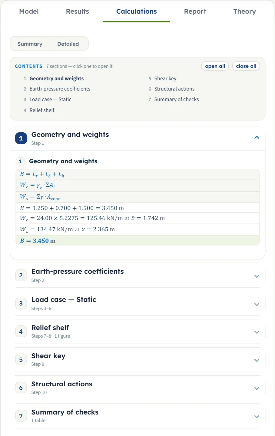
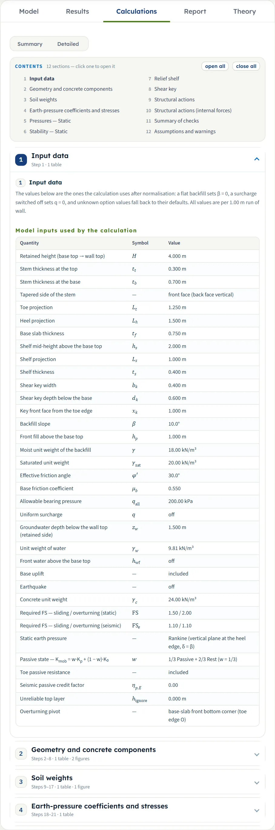
The Calculations tab has two levels, Summary and Detailed, chosen with the buttons at the top, and a contents list whose sections open and close (open all, close all). Summary has seven sections: Geometry and weights, Earth-pressure coefficients, one section for each load case, Relief shelf, Shear key, Structural actions and Summary of checks. Detailed has twelve and 42 steps: Input data, Geometry and concrete components, Soil weights, Earth-pressure coefficients and stresses, Pressures for each case, Stability, Relief shelf, Shear key, Structural actions, the internal forces, Summary of checks, and Assumptions and warnings. Each step shows the equation, the numbers substituted and the result. Before Analyze the tab says “Press Analyze on the Model tab to calculate this wall.”
The Report
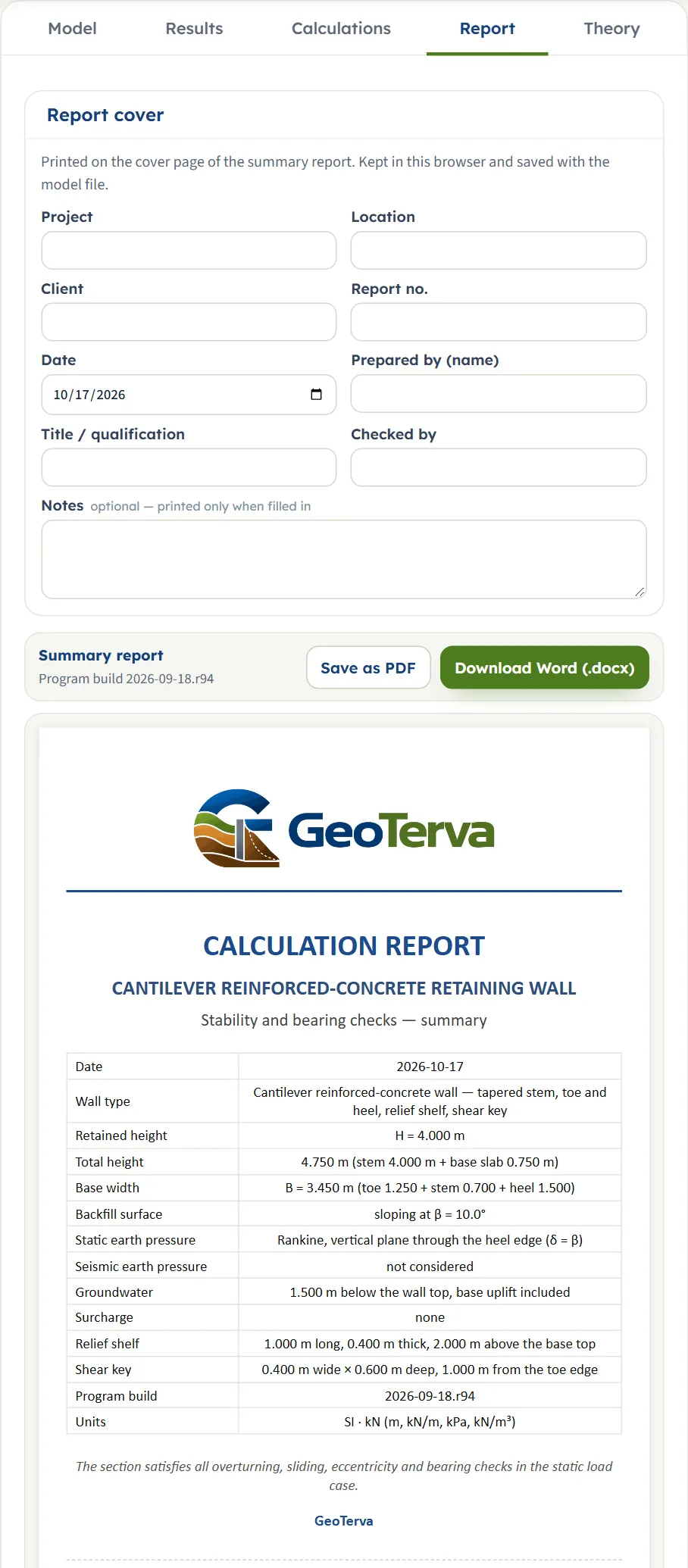
The Report tab has a cover form (project, location, client, report number, date, prepared by, title or qualification, checked by and optional notes), kept in the browser and saved with the model file. After Analyze, Save as PDF (it opens a print window: choose Save as PDF there) and Download Word (.docx) are available; before it they are greyed out. The preview is the summary report.
It has thirteen parts: 1 Purpose and scope, 2 Design basis and assumptions, 3 Geometry and section, 4 Soil, material and load parameters, 5 Resisting forces, 6 Lateral earth pressure coefficients, 7 Driving forces, 8 Overturning check, 9 Sliding check, 10 Eccentricity and base pressure, 11 Relief shelf and shear key, 12 Design actions for the RC members and 13 Summary of results, with the drawings and the tables. When the run carries cautions, a part with them is added.
The Theory tab
The Theory tab explains the method in 21 sections: Overview; The wall system; Coordinates and signs; Geometry decomposition; Soil moving with the wall; Effective stress; Rankine; Coulomb; At-rest and passive resistance; Surcharge; Hydrostatic water and uplift; Mononobe–Okabe; Hydrodynamic water; Inertia of wall and soil; Relief shelves; Shear keys; Sliding, overturning, bearing; Structural actions; Worked example; Variables; References.
Worked example: the module’s own example
The module opens on this example; you can follow every number on your own screen (values from the Calculations tab, SI · kN).
| Section | Inputs |
|---|---|
| Geometry | H = 4.00 m; stem 0.30 m at the top and 0.70 m at the base, thickening toward the front; toe 1.25 m, heel 1.50 m, slab 0.75 m |
| Optional geometry | Shelf: hs = 2.00, Ls = 1.00, ts = 0.40 m. Key: 0.40 m wide, 0.60 m deep, 1.00 m from the toe edge |
| Backfill, front fill | Inclined, β = 10°; hp = 1.00 m |
| Soil | γ = 18, γsat = 20 kN/m³, φ′ = 30°, μb = 0.55, qall = 200 kPa |
| Water | Retained side zw = 1.50 m below the wall top; no front water; uplift included |
| Settings | Rankine; 1/3 Passive + 2/3 Rest; toe passive on; no earthquake; required FSs = 1.50, FSo = 2.00 |
Step 1: the coefficients
The Rankine coefficient for β = 10° and φ′ = 30° is Kaβ = 0.3495 along the slope, and the horizontal part is Ka = 0.3495 cos 10° = 0.3442, the value the module shows. Kp = tan²60° = 3.0000, K0 = 1 − sin 30° = 0.5000, Kmob = ⅓ · 3.0000 + ⅔ · 0.5000 = 1.3333.
Step 2: weights and forces
- Concrete Wc = 24.00 × 5.2275 = 125.46 kN/m; soil moving with the wall Ws = 134.47 kN/m; their sum 259.93 kN/m.
- Water on the plane: the water column from the water table to the base underside is 3.25 m, so Pw = ½ · 9.81 · 3.25² = 51.81 kN/m. Soil thrust Pa,H = 36.77 kN/m (it is relieved by the shelf, R = 0.789). Hdrive = 36.77 + 51.81 = 88.58 kN/m.
- Passive: Ptoe = Kmob γ Df² / 2 = 1.3333 × 18 × 1.75² / 2 = 36.75 kN/m; Pkey = (42.00 + 56.40)/2 × 0.60 = 29.52 kN/m.
- Normal force: Neff = 259.93 + Pa,V 6.48 − uplift 57.35 = 209.06 kN/m.
Step 3: the four checks
- Sliding: FSs = (0.55 × 209.063 + 36.75 + 29.52) / 88.584 = 2.046 ≥ 1.50, OK.
- Overturning about the toe edge: FSo = 558.89 / 265.94 = 2.102 ≥ 2.00, OK.
- Eccentricity: xR = (558.89 − 265.94) / 209.06 = 1.401 m, so |e| = 1.725 − 1.401 = 0.324 m ≤ B/6 = 0.575 m, OK.
- Bearing: qmax = 209.06 / 3.45 × (1 + 6 × 0.3238 / 3.45) = 94.72 kPa ≤ 200 kPa, OK; qmin = 26.48 kPa, full contact.
These are the numbers of the Results tab. The soil weights and the uplift are read from the module; the rest follow from them by the formulas above.
A plain wall, checked by hand
Switch the shelf, the key, the water, the front fill and the uplift off and choose Flat: the wall is a plain 4 m wall on a 3.45 m base. Then Ka = ⅓; the plane is 4.75 m high, so Pa = ½ · ⅓ · 18 · 4.75² = 67.69 kN/m at 1.583 m; the weights are 218.10 kN/m (concrete and the soil over the heel); the toe passive is 1.3333 · 18 · 0.75² / 2 = 6.75 kN/m. Sliding: (0.55 × 218.10 + 6.75) / 67.69 = 1.872; overturning: 479.68 / 107.17 = 4.476; |e| = 0.017 m and qmax = 65.09 kPa. The stem at its base carries V = ½ · ⅓ · 18 · 4² = 48.00 kN/m and M = 48.00 × 4/3 = 64.00 kN·m/m. The module gives the same numbers. An independent calculation also agrees with the module for a sloping backfill, a different soil, a uniform surcharge, the front fill, hignore, the passive states, the toward-backfill and the constant stem, and the seismic cases below.
The seismic cases of the plain wall
Add the earthquake with kh = 0.15 and kv = 0.10 (η = 0, so no passive credit). Mononobe–Okabe with ψ = arctan(kh / (1 ∓ kv)) gives Kae = 0.4459 (vertical acceleration upward) and 0.4227 (downward); PAE = ½ γ (1 ∓ kv) Kae h² = 81.49 and 94.41 kN/m. With the inertia kh W = 32.72 kN/m the horizontal force is 114.21 and 127.12 kN/m, the normal force (1 ∓ kv) W is 196.29 and 239.91 kN/m, and sliding is 0.55 × 196.29 / 114.21 = 0.945 and 0.55 × 239.91 / 127.12 = 1.038. The module gives the same.
The same wall in the other unit systems
In SI · tf the example gives qmax = 9.66 t/m² against a limit of 20.39 t/m², the earth thrust 3.75 tf/m, the water force 5.28 tf/m and the concrete unit weight 2.45 t/m³; in US, qmax = 1.98 ksf against 4.18 ksf, 2.52 and 3.55 kip/ft, and H reads 13.12 ft. The factors 2.05 and 2.10 are the same in the three systems; the eccentricity reads 0.324 m, 0.324 m and 1.062 ft, against a limit of 0.575 m and 1.886 ft.
How each input changes the answer
Each row changes one thing in the example (H = 4 m, β = 10°, γ = 18, γsat = 20 kN/m³, φ′ = 30°, μb = 0.55, shelf, key, water at 1.5 m and uplift as in the Worked example). The second column gives the static sliding factor and the static overturning factor, the third the largest base pressure in kPa and the eccentricity in m. The numbers are the ones the module gives, so you can reproduce any row.
| Change | FSs / FSo | qmax kPa / |e| m |
|---|---|---|
| The example Rankine; Coulomb gives the same | 2.05 / 2.10 | 94.72 / 0.324 |
| Flat backfill β = 0 | 2.26 / 2.17 | 87.64 / 0.299 |
| β = 20° | 1.79 / 2.01 | 106.18 / 0.356 |
| φ′ = 35° | 2.43 / 2.25 | 85.73 / 0.246 |
| φ′ = 25° overturning below 2.00 | 1.73 / 1.95 | 105.98 / 0.419 |
| γ = 20, γsat = 21 kN/m³ | 2.11 / 2.13 | 99.14 / 0.316 |
| H = 3 m | 3.36 / 3.07 | 58.26 / 0.057 |
| H = 5 m three checks not satisfied | 1.38 / 1.52 | 163.08 / 0.756 |
| Heel 2.00 m | 2.27 / 2.41 | 86.22 / 0.233 |
| Heel 1.00 m | 1.82 / 1.75 | 109.70 / 0.460 |
| Toe 0.50 m partial contact | 1.95 / 1.72 | 160.25 / 0.543 |
| Base slab 0.50 m | 2.03 / 2.22 | 78.52 / 0.236 |
| Stem thickening toward the backfill | 2.04 / 2.13 | 105.91 / 0.354 |
| Constant stem, 0.50 m | 2.04 / 2.03 | 108.24 / 0.376 |
| Shelf off | 1.58 / 1.90 | 109.39 / 0.448 |
| Key off | 1.69 / 2.10 | 92.83 / 0.320 |
| Shelf and key off | 1.31 / 1.90 | 107.50 / 0.446 |
| Water off | 4.45 / 6.01 | 78.18 / 0.018 |
| Water table at the wall top, zw = 0 | 1.21 / 1.34 | 160.34 / 0.948 |
| Uplift off | 2.40 / 4.09 | 96.02 / 0.140 |
| Front water 0.50 m overturning below 2.00 | 1.88 / 1.94 | 81.92 / 0.284 |
| No front fill, hp = 0 | 1.40 / 2.04 | 75.26 / 0.229 |
| μb = 0.45 only sliding changes | 1.81 / 2.10 | 94.72 / 0.324 |
| Full Rest passive state | 1.58 / 2.10 | 94.72 / 0.324 |
| Toe passive off | 1.63 / 2.10 | 94.72 / 0.324 |
- Water has the largest effect among the rows above: with the water switched off the sliding factor is 4.45 and the overturning factor 6.01; with the water table at the wall top they fall to 1.21 and 1.34, and the eccentricity reaches 0.948 m, outside B/6 = 0.575 m. The uplift acts the same way.
- Height matters steeply: the thrust grows with H². From 3 m to 5 m the sliding factor goes from 3.36 to 1.38.
- The heel helps overturning and eccentricity more than sliding: 1.00 m to 2.00 m raises FSo from 1.75 to 2.41. A longer toe lowers the largest base pressure: 160.25 kPa with a 0.50 m toe, 94.72 kPa with 1.25 m.
- Only sliding responds to μb, the passive state, the toe switch and hignore: the overturning, the eccentricity and the bearing pressure do not use the passive resistance.
- The concrete strength, the yield strength and the cover change nothing; γc changes the weights (2.08 for 25 kN/m³).
- qall changes only the verdict: with 100 kPa the pressure of 94.72 kPa still passes, with 50 kPa it does not.
Messages: when the module stops, and what it warns about
Stops
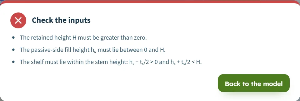
When an input cannot be used, Analyze opens a window and nothing is calculated. A missing or out-of-range value gives Check the inputs, a bullet list of every message that applies, and the button Back to the model. A geometry or method that has no solution gives The wall could not be analysed with one message. The bar stays on Not analysed.

| When | Message |
|---|---|
| H is zero or empty | “The retained height H must be greater than zero.” (with it, the shelf and hp messages below usually follow) |
| Stem thickness is zero, or the base thinner than the top | “The stem thickness must be greater than zero.” / “The stem base thickness tb must be at least the top thickness tt.” |
| Toe, heel or slab out of range | “The toe projection Lt must be zero or more.” / “The heel projection Lh must be zero or more.” / “The base slab thickness tf must be greater than zero.” |
| β outside −45° to 45° | “The backfill slope β must lie between −45° and 45°.” |
| hp above H | “The passive-side fill height hp must lie between 0 and H.” |
| Unit weights | “Enter a positive moist unit weight γ.” / “Enter a positive saturated unit weight γsat.” / “γsat must exceed the water unit weight γw.” / “Enter a positive concrete unit weight γc.” |
| φ′ outside 0° to 60° | “The friction angle φ′ must lie between 0° and 60°.” |
| μb or qall not positive | “The base friction coefficient μb must be greater than zero.” / “The allowable bearing pressure must be greater than zero.” |
| A required factor not positive | “The stability criteria must be positive.” |
| Water | “The groundwater depth zw must be zero or more.” / “The front water height hwf must be zero or more.” |
| Shelf | “The shelf projection Ls and thickness ts must be greater than zero.” / “The shelf must lie within the stem height: hs − ts/2 > 0 and hs + ts/2 < H.” |
| Key | “The key width bk and depth dk must be greater than zero.” / “The key must lie under the base: 0 ≤ xk and xk + bk ≤ B.” |
| Earthquake | “kh must lie between 0 and 1.” / “kv must lie between 0 and 1.” |
| Passive settings | “The seismic passive credit factor ηp,E must lie between 0 and 1.” / “The unreliable top layer hignore must be zero or more.” |
| A surcharge load is not usable | “Strip load 1: the load q must be zero or more.” / “Strip load 1: the near edge x₁ must be zero or more.” / “Strip load 1: the far edge x₂ must be greater than the near edge x₁.” / “Point load 2: the load Q must be zero or more.” / “Point load 2: the distance x from the wall must be zero or more.” (the number is the place of the load in the table). When you press Add load on an incomplete form, the form itself says, for example, “The new load: the far edge x₂ must be greater than the near edge x₁.” |
| The backfill falls below the base slab at the heel | “The backfill surface must stay above the base slab at the heel.” |
| The size of β not below φ′ (Rankine) | “No real Rankine inclined-backfill solution for the entered β and φ′ (β must be smaller than φ′).” |
Where several values are wrong, all their messages are listed together. An empty box in a required field gives the message of that field.
Warnings
Analysis runs, and the cautions are listed in the Attention window, in the Warnings (N) list and at the top of the Results tab. Each has a reason and a remedy:
| Warning | Reason and remedy |
|---|---|
| Sliding or overturning factor of safety below the requirement (static or the seismic case) for example “FS = 1.38 < 1.50.” | Remedy: “Add or deepen a shear key, widen the base or increase the front resistance.” for sliding; “Lengthen the heel or the toe.” for overturning. A factor that is below its requirement never prints equal to it: when both round to the same two decimals, more decimals are shown, so for H = 4.7675 m in the example the text reads “FS = 1.4996 < 1.5000.” and the Sliding card shows 1.4996 / 1.5000. |
| Partial base contact | “The resultant lies outside the middle third, so part of the base lifts off.” Remedy: “Lengthen the base or the heel, or reduce the lateral load.” |
| Bearing pressure exceeds the allowable value | The largest pressure is above qall. Remedy: “Widen the base or reduce the loads.” |
| The seismic load cases are not evaluated | “No real Mononobe–Okabe equilibrium solution: the thrust has no maximum …” for kh = 0.6, for example. Remedy: “Change the soil and seismic parameters under Analysis Settings. The static case below is unaffected.” |
| Load case “Static” is not covered by the design envelope | “Its resultant falls outside the base, so it has no contact pressure and no design actions …” The case has no bearing value (“cannot be evaluated” in the Results tab). |
| The shelf tip reaches beyond the external pressure plane | “The relief shelf is wider than the heel, which the relief method does not cover.” Remedy: shorten the shelf or lengthen the heel. |
| Front water height exceeds the passive-side soil height | “The water in front of the wall stands above the front fill.” |
| The retained groundwater table is above the ground | “The groundwater table lies above the backfill surface at the heel, so free water would stand on the ground.” |


Good practice and common mistakes
- Know what the plane is. The earth pressure acts on the vertical plane through the heel edge, and the soil between the stem and that plane is counted as weight. The thrust is parallel to the backfill, so a sloping backfill adds a vertical part Pa,V to the normal force.
- Use the passive resistance with care. It is credited in sliding only. Start from the default state (1/3 passive), switch the toe off if the front soil may be removed (or enter hp = 0), and use hignore for frost, erosion or a future trench.
- Give the water its real level. Water behind the wall raises the thrust and the uplift; in the example it lowers the sliding factor from 4.45 to 2.05.
- Check the shelf against the heel. The relief method assumes the shelf is no wider than the heel; the module warns when it is.
- Choose the earthquake coefficients yourself. The module applies the kh and kv you enter and runs both vertical directions; the passive credit ηp,E is 0 until you decide otherwise.
- Read the governing case. On the cards and in the table the governing case of each check is outlined.
- Use the actions for the reinforcement. The stem, toe, heel, shelf and key moments and shears are the inputs of the section design.
- Enter loads in the unit system you chose. A strip or point load is measured from the back face of the wall at its top.
- Keep a record. The report, a saved model file or a Quick Save keep what an analysis was based on.
Frequently asked questions
What does the Cantilever RC wall module check?
Sliding, overturning, eccentricity and bearing pressure of a reinforced-concrete cantilever wall, static and seismic, and the shear and moment in its stem, toe, heel, shelf and key. The example gives sliding 2.05, overturning 2.10, a largest base pressure of 94.72 kPa and an eccentricity of 0.324 m.
Why is the earth pressure taken on a vertical plane through the heel?
The wall is treated with the soil over the heel as one body: the thrust acts on the vertical plane through the heel edge, soil against soil, parallel to the backfill surface, and that soil is counted as weight. For this plane Rankine and Coulomb give the same coefficient.
Is there a difference between Rankine and Coulomb here?
No: for a vertical plane with the wall friction angle equal to β the Coulomb coefficient equals the Rankine one, and the example gives the same factors with either choice.
What is the pressure-relief shelf and what does the module do with it?
A horizontal slab on the back of the stem. Below its underside the soil self-weight pressure restarts and is reduced by R = min(Ls / bkr, 1). The relieved pressure is used on the stem and on the external plane; the surcharge and the water are not reduced. In the example R = 0.789 and the stem base moment falls from 84.63 to 69.62 kN·m/m.
What does the shear key add?
The passive resistance Pkey of the soil in front of the key is added to the sliding resistance. In the example the sliding factor is 2.05 with the key and 1.69 without it; the key weight still counts in the weights.
Is the passive resistance used in overturning and bearing?
No, in sliding only. That is why the passive state, the toe switch and hignore change the sliding factor and nothing else.
Do f′c, fy and the cover change the results?
No. They are kept with the model; only the concrete unit weight enters the weights. The stem and slab actions are given for your reinforcement design.
How does the earthquake work?
With Earthquake Yes the module runs Mononobe–Okabe for the soil, the hydrodynamic water pressure and the inertia of the wall and the soil that moves with it, for the vertical acceleration upward and downward, and reports each case; the lower factor governs. The seismic passive credit is ηp,E, 0 by default.
What values does the module accept?
For example H above zero, the size of β above −45° and below 45° and below φ′, φ′ from above 0° to below 60°, hp from 0 to H, kh and kv from 0 to below 1; the full list is in Messages. A missing or out-of-range value stops the analysis with a message that names it.
Can I drag the wall or the loads on the drawing?
No dragging of the section: change the values in the Model tab. The 3D View rotates by dragging, and double-clicking resets it. After Analyze the inputs are locked until you press Edit inputs.
Does the module remember my inputs?
Yes. Every change is kept in the browser and the page opens on the model you last worked on, analysed if it was. Reset to defaults brings back the example; Save to file and Quick Save keep copies.
What does the report contain?
A cover with your project details, then thirteen parts from the purpose and the design basis to the summary of results, with the drawings, saved as a PDF or a Word file after Analyze.