

What the module calculates
Slope stability gives the factor of safety of a slope by the limit-equilibrium method of slices. You draw a section (the ground surface, layers of soil or rock, groundwater, loads, reinforcement), choose a method, and the module cuts many slip surfaces out of the slope, analyses every one and keeps the lowest factor of safety: the critical surface. The section is two-dimensional: every force is per metre of its length.
- Ground: layers bounded by lines of points, each layer with a material that is drained (c′, φ′), undrained (cu, which may grow with depth) or a rock mass (Hoek–Brown criterion).
- Water: a water line of any shape, ponded water, a pore pressure ratio ru per material, and a rapid drawdown.
- Loads: strip loads and point (line) loads on the ground surface, vertical, normal or at an angle.
- Reinforcement: soil nails, ground anchors and geogrids.
- Earthquake: a pseudo-static analysis with kh and kv that you give.
- Methods: the ordinary method of slices (Fellenius), Bishop simplified, and Spencer (forces and moments). Circular slip surfaces come from a grid of centres; a non-circular surface is searched as a polyline and analysed by Spencer.
- Input aids: a DXF drawing can be imported (the module tells how to draw it and has example files to download), and the Measure tools put dimensions on the drawing.
For a plane failure surface parallel to the ground use Infinite slope.
Before you start: what you need
| What | Notes |
|---|---|
| The section | The ground surface as points x, z in metres, left to right, and the level zbase below which no slip surface passes (it must lie below the lowest ground point). |
| The layers | The lines between the layers and a material for each layer. |
| The strength of each material | Unit weights γ and γsat and c′, φ′ (or cu, or the rock parameters). |
| Water, loads, reinforcement | Only if they exist on your site. |
| kh, kv | Only for a pseudo-static case; the module takes them as inputs. |
Quick start in seven steps
- Draw the ground surface
In Ground surface type the points or drag them on the drawing; set the base zbase.
- Add layer boundaries and materials
Add boundaries in Layer boundaries, create materials in Materials and give each layer one in Assign materials.
- Add water, loads, reinforcement, earthquake
Use Groundwater, Loads, Soil nails, Ground anchors, Geogrids and Earthquake as the site requires.
- Set the search
In Slip surfaces place the rectangle of centres (the Suggest a rectangle button gives a start). In Analysis choose the method and the slicing.
- Check the model
Press Model check to see errors, warnings and notes.
- Press Analyze
The module analyses every circle of the grid, switches to the Results tab and shows the factor of safety. The model is locked until you press Edit inputs.
- Read and report
Press a slice for its working, read the Calculations tab, and take the Report as PDF or Word.
The screen: tools, chips and dragging
The layout is the shared one described in the workspace guide: the drawing on the left and five tabs on the right: Model, Results, Calculations, Report and Theory. When you press Analyze the module moves to Results by itself.
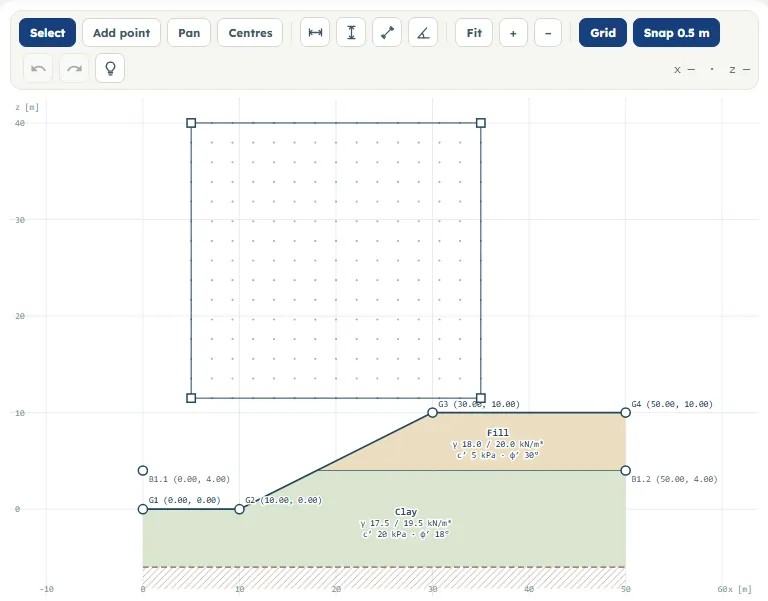
The tools
- Select: press a point, a boundary, the water line, a layer, a load or a reinforcement element to select it and open its row on the Model tab; drag a point to move it.
- Add point: press a line (ground, boundary, water line, slip surface) to insert a point there.
- Pan: drag the drawing; the wheel zooms in any tool; Fit, + and − also zoom.
- Centres: drag a rectangle; the centres of the slip circles are the points of a grid inside it. The tool returns to Select when the rectangle is drawn.
- The four Measure buttons: a horizontal, a vertical and an aligned dimension (two points each) and an angle (the vertex, then a point on each line). A measure lands on a point of the section when one is within ten pixels; Esc drops it. A distance reads like 20.000 m and an angle like 153.4°. Press a dimension to select it and press Delete to remove it. The dimensions are shown with the Dimensions chip, which switches itself on when you make one.
- Grid shows the grid lines; Snap 0.5 m makes dragged points land on 0.5 m (switched off, they land on 0.01 m).
- Undo and redo (Ctrl+Z, Ctrl+Y) keep the last 60 changes. Delete removes the selected point, load, reinforcement element or dimension.
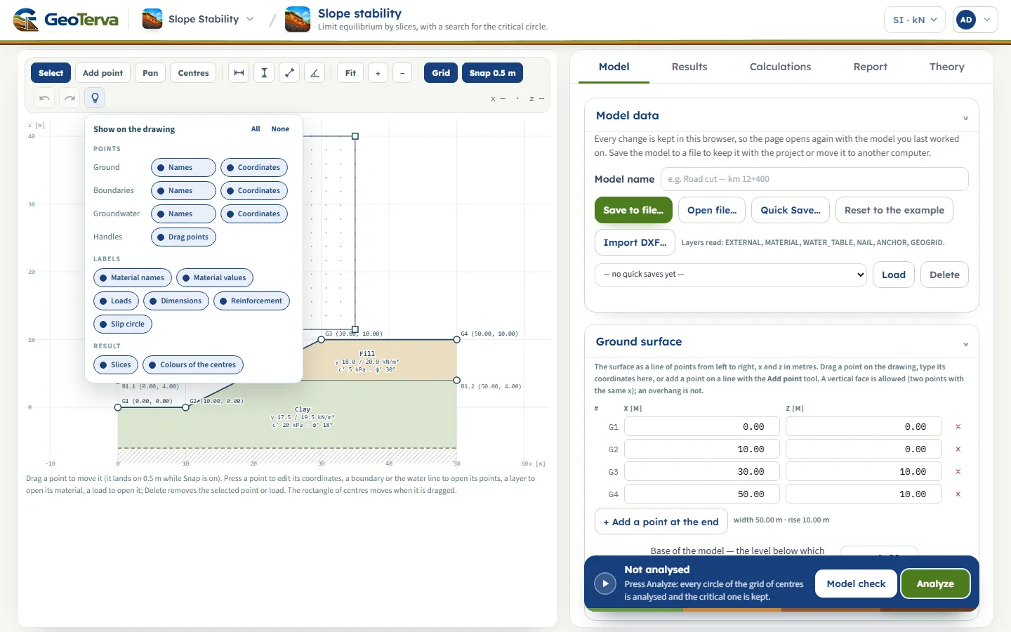
The bulb: what the drawing shows
The bulb opens Show on the drawing, with All and None. Points: names and coordinates of the ground, boundaries and groundwater, and the Drag points handles. Labels: Material names, Material values, Loads, Dimensions, Reinforcement, Slip circle. Result: Slices and Colours of the centres. The choice is kept by the browser. After Analyze the point labels are hidden for a clear drawing; press a chip to bring them back.
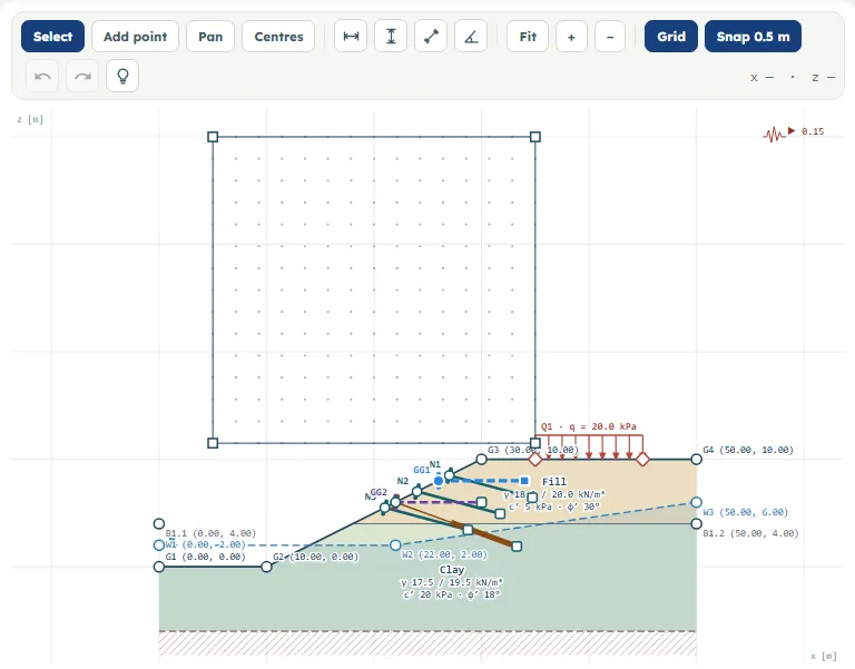
Dragging
- Points of the ground, a boundary, the water line or a polyline slip surface move with the pointer; a point stays between its neighbours in x, so a line remains a function of x. Double-click a point to remove it (a line keeps at least two points).
- A strip load has two ends and a point load one, dragged along the surface; a load keeps its place on the surface when the ground is edited.
- A reinforcement element has two handles: the head moves along the surface; the tip turns and lengthens it (a geogrid stays horizontal).
- The rectangle of centres moves when dragged and is resized by its corners.
- After Analyze the model is locked: nothing is dragged, but pan, zoom and selecting a slice still work. Edit inputs unlocks it.
Entering the model, section by section
The Model tab starts with Model data, which stands apart; then twelve sections walked one at a time (the one open carries Back and Next): Ground surface, Layer boundaries, Materials, Assign materials, Groundwater, Loads, Soil nails, Ground anchors, Geogrids, Earthquake, Slip surfaces, Analysis. A box takes its value when you press Enter or leave it.
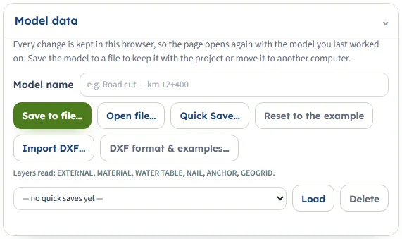
Model data: keeping the model
Every change is kept by the browser, so the page opens on the model you last worked on; the line under the buttons says so and gives the time it was kept. The analysed state is not kept: you press Analyze again. Buttons: Save to file… (a .gtrv file named after the model name, with the report cover details inside; a browser without a save window puts it in its downloads folder), Open file…, Quick Save… (asks for a name; a name already in use asks whether to replace it; the saved versions are in the list, with Load and Delete), Reset to the example (asks first, and clears the model name) and Import DXF…, with DXF format & examples… beside it. While the model is locked after an analysis, Open file…, Load, Delete and Reset to the example are off, and the DXF button is off too (its tooltip says to press Edit inputs first): press Edit inputs first. DXF format & examples… stays on.
DXF import. The layers read are EXTERNAL (one closed line: the ground surface, the two sides and the base), MATERIAL (the lines between soils), WATER TABLE (a space, a hyphen or an underscore between the words is accepted), NAIL, ANCHOR (three points: head, end of the free length, tip) and GEOGRID; LINE, LWPOLYLINE and POLYLINE entities are read. A window then lists what was read, for example: the ground surface with 4 points, 1 layer boundary (2 layers), the water table with 3 points, the base of the model at z = −6 m; the reinforcement found (1 soil nail, 1 ground anchor, 1 geogrid, whose place and direction come from the drawing and whose capacities are starting values); and the layers of the drawing that were not read. Every region gets a soil of its own (γ 18 / 20 kN/m³, c′ 5 kPa, φ′ 30°) for you to rename and edit. The import replaces the whole model, loads and earthquake included, and Undo brings the old one back. Without an EXTERNAL layer the module says so and lists the layers in the file, with a button to the format notes described next.
DXF format and examples. DXF format & examples…, beside Import DXF…, opens a window that tells how the section is drawn: a table of the six layers (EXTERNAL is required, the others only when the section has them) with the other names that are read for each, and the rules: capitals, spaces, hyphens and underscores do not matter; LWPOLYLINE, POLYLINE and LINE entities are read, arcs, splines and blocks are not; only x and y are used, as metres; the other layers of the drawing are ignored. Under them are three example drawings, each with its layers in colour and a button that saves its file: a slope on two soils with a water table, a cut held by soil nails and a ground anchor, and an embankment with geogrids. The files are DXF drawings of release 12, which every CAD program opens: open one to see how the layers are used, then draw your own section the same way. Import DXF… reads each of them as it is.
Ground surface
A line of points from left to right. A vertical face (two points with the same x) is allowed; an overhang is not.
+ Add a point at the end adds a point 5 m on; × removes a point (two remain at least). The line under the points gives the width and the rise.
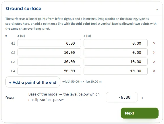
| Field unit | Default |
|---|---|
| Point x, zm | G1 (0, 0), G2 (10, 0), G3 (30, 10), G4 (50, 10) |
| zbase base of the modelm | −6 |
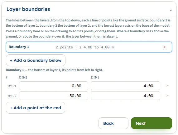
Layer boundaries and Assign materials
Boundary k is the bottom of layer k; the lowest layer rests on the base. + Add a boundary below puts a level boundary half-way between the lowest ground and the base (z = −3 m on the example); the new layer takes the material of the layer above it. Press a boundary to edit its points; × removes it (the layer above extends down). Where a boundary rises above the ground, that layer is absent there: the example has this, and the module notes it as INFO. Assign materials has one row per layer with a material list.
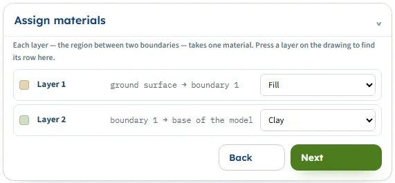
Assign materials has one row per layer: the layer, the two boundaries it lies between (the lowest rests on the base of the model) and its material. Press a layer on the drawing to find its row.
Materials
Choose the Strength: Drained — c′ and φ′, Undrained — cu, φ = 0 or Rock — Hoek–Brown, fill the form and press + Add material; press a row of the table to change it (changes apply as they are entered); × deletes a material not used by a layer.
Drains freely in a rapid drawdown is a switch per material. A name is automatic when left empty; the colour is chosen on the form. The example holds Fill (18 / 20, c′ 5, φ′ 30) and Clay (17.5 / 19.5, c′ 20, φ′ 18).
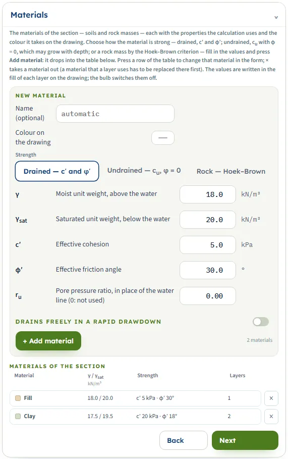
| Field unit | Default of a new material |
|---|---|
| γ moist unit weightkN/m³ | 18 |
| γsat saturatedkN/m³ | 20 |
| c′kPa | 5 |
| φ′°, 0 to 60 | 30 |
| cu (undrained)kPa | 50 |
| k: growth of cu per metre below level zkPa/m | 0 |
| z level at and above which cu is as givenm | 10 |
| σci (rock)MPa | 20 |
| GSI (rock)5 to 100 | 45 |
| mi (rock) | 10 |
| D (rock)0 to 1 | 0 |
| ru pore pressure ratio0 to 0.95; 0 = not used | 0 |
Groundwater
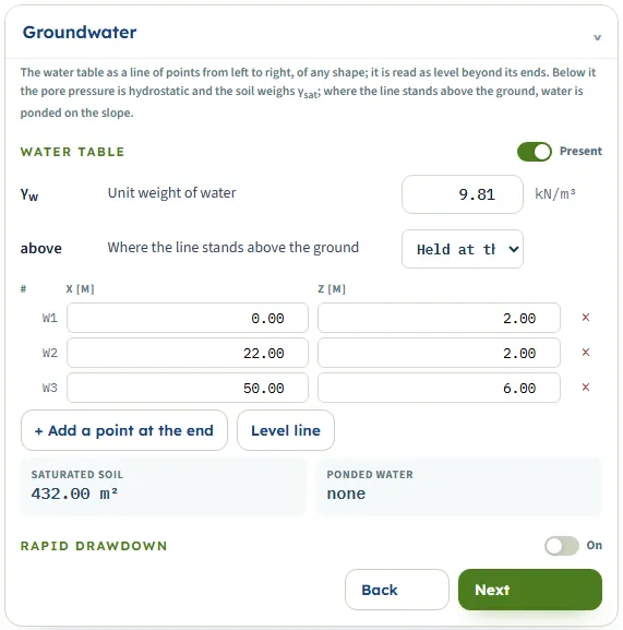
Switch Present on for a water line (points left to right, any shape, level beyond its ends); Level line makes a level line a little over a third of the way up the surface. γw is an input (9.81 kN/m³). Where the line stands above the ground is either “Held at the ground surface — no water on the slope” or “Ponded water on the slope — its weight and pressure act”. Below the line the pressure is hydrostatic and the soil weighs γsat; with ponded water the water standing on the slope adds its weight as a vertical load and its pressure against the rising ground as a horizontal one, and the pore pressure at the base is measured up to the line. Rapid drawdown (on/off, level zdd) takes the line as the state before the water falls.
Loads
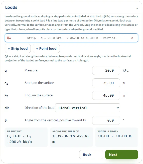
+ Strip load (q in kPa between two points x₁, x₂ of the surface) and + Point load (P in kN/m at one point). New loads sit on the crest (strip 20 kPa across the middle half; point 100 kN/m at its middle). The direction is “Global vertical”, “Normal to the surface” or “At an angle from the vertical” (θ, positive toward +x; a value outside −89° to 89° is an error in the model check). A strip load acts on the horizontal projection of the loaded surface; a normal one on its length.
Soil nails, ground anchors, geogrids
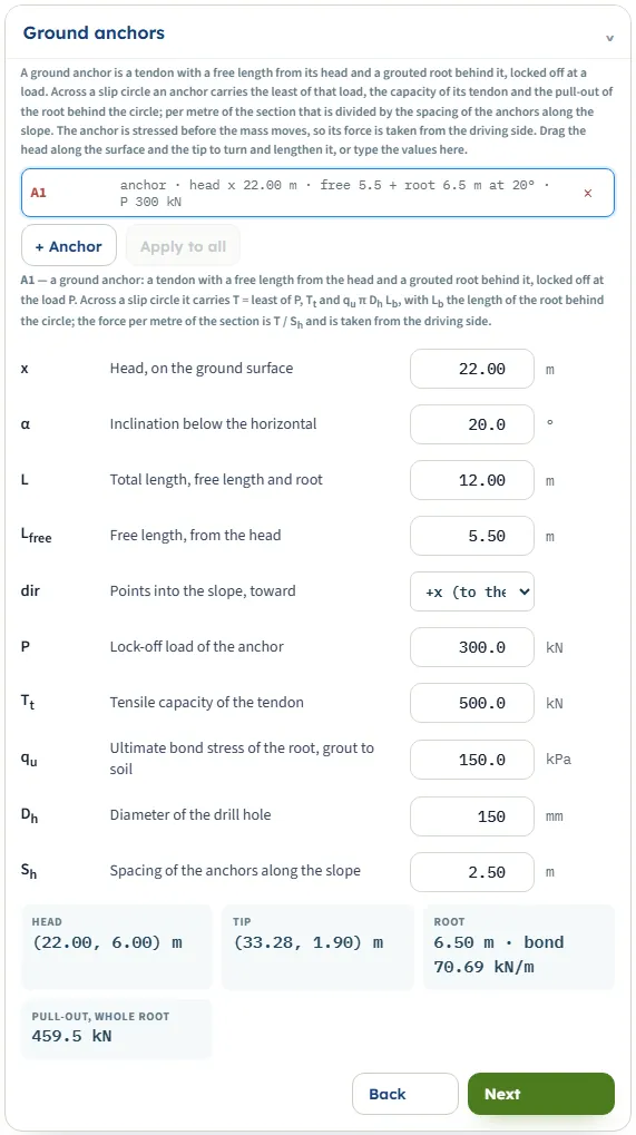
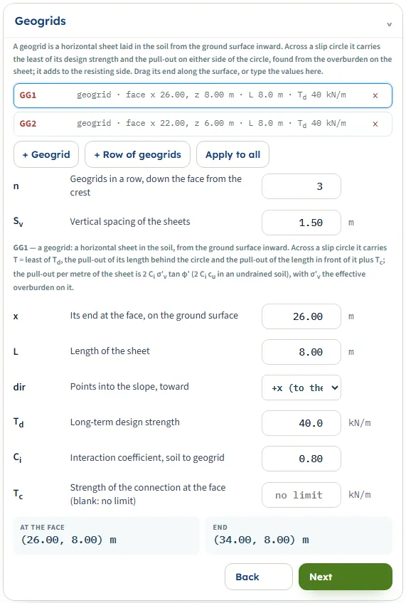
+ Soil nail, + Row of nails (n nails down the face at vertical spacing Sv; defaults 3 and 1.5 m), + Anchor, + Geogrid, + Row of geogrids; Apply to all copies the angle, length, free length, load, capacities, bond, hole diameter and spacing of the selected element to the others of its kind (not the head position or the direction). A new nail is put on the face 1.5 m under the crest and each row continues down the face: a row of 3 on the example with no nails yet gives heads at x = 27, 24 and 21 m.
Each element also has its head x on the ground and a direction (toward +x or −x). A nail carries the least of the bar tension, the pull-out behind the circle and the pull-out in front plus the head; an anchor the least of P, Tt and the root pull-out, taken from the driving side; a geogrid the least of Td and the two pull-outs. The force is per metre of section: T / Sh (a geogrid is already per metre). An element whose tip lies inside the sliding mass, or whose head lies outside it, carries nothing on that circle.
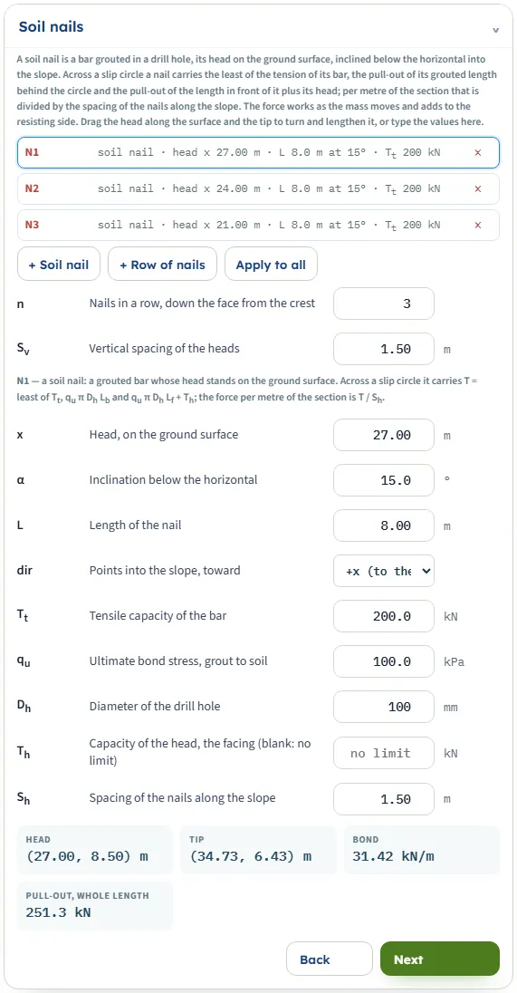
| Element | Defaults |
|---|---|
| Soil nail | α 15°, L 8 m, Tt 200 kN, qu 100 kPa, Dh 100 mm, Th no limit, Sh 1.5 m |
| Anchor | α 20°, L 12 m and free length 5.5 m on the example slope (about 1.2 times the height, 45 % free), P 300 kN, Tt 500 kN, qu 150 kPa, Dh 150 mm, Sh 2.5 m |
| Geogrid | L 8 m, Td 40 kN/m, Ci 0.8, Tc no limit |
A ground anchor has the length, the free length, the lock-off load P and the capacity of the tendon; the section shows the head, the tip, the root and its bond, and the pull-out of the whole root (459.5 kN for the default anchor on the example). A geogrid has its end at the face, the length, the design strength Td, the interaction coefficient Ci and the strength of the connection Tc; it is horizontal.
Earthquake
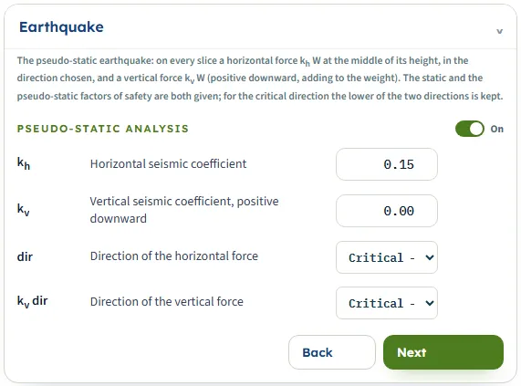
Switch Pseudo-static analysis on. kh (0 to 1, default 0.15), kv (−0.5 to 0.5, positive downward, default 0), the direction of the horizontal force (Critical — the lower factor of the two directions, toward −x, toward +x) and of the vertical force (critical, downward, upward). The static and the pseudo-static factors are both given. You choose kh and kv yourself; the module applies no code.
Slip surfaces
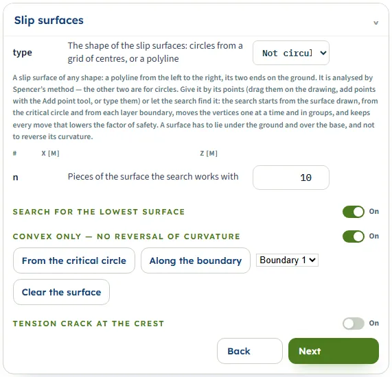
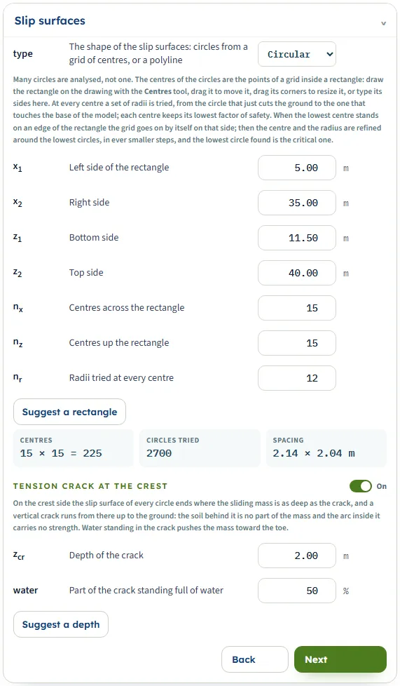
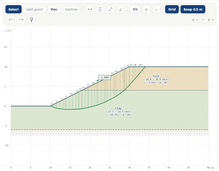
Circular (default): the rectangle x₁, x₂, z₁, z₂ and the numbers of centres across (nx) and up (nz), 2 to 81 (default 15 × 15), and the radii at every centre nr, 3 to 40 (default 12). Drag it with Centres, or Suggest a rectangle. The example rectangle is x 5 to 35, z 11.5 to 40. The grid widens by itself when the lowest centre stands on an edge. Not circular: a polyline of points (ends on the ground), analysed by Spencer; Search for the lowest surface is on by default, Convex only — no reversal of curvature too; n = 3 to 30 pieces (10); From the critical circle, Along the boundary (with a boundary list) and Clear the surface give starts.
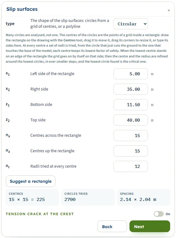
Tension crack at the crest: depth zcr (default 2 m) and the part full of water in percent (default 0, 0 to 100); Suggest a depth gives 2c′/γ · tan(45° + φ′/2) of the soil at the crest, or 2cu/γ undrained (1.0 m for the Fill of the example, 4.4 m if the Fill were undrained with cu 40 kPa). The slip surface of every circle ends where the mass is as deep as the crack; the arc inside the crack carries no strength.
Analysis
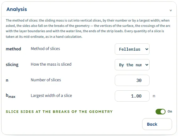
method: Fellenius (default), Bishop simplified, Spencer. slicing: by number (5 to 200, default 30) or by a largest width (default 1 m). Slice sides at the breaks of the geometry (on by default): vertices of the surface, crossings of the arc with boundaries and the water line, ends of strip loads become slice sides. A non-circular surface is always analysed by Spencer, and the method list is disabled.
Choosing the method
| Method what it satisfies | Factor on the example circle |
|---|---|
| Fellenius (ordinary)Moments of the whole mass; the forces between slices are neglected | 1.569 |
| Bishop simplifiedVertical equilibrium of each slice and moments; the shear between slices neglected; found by iteration | 1.740 |
| SpencerForces and moments, with one angle θ for the forces between slices (18.54° here) | 1.717 |
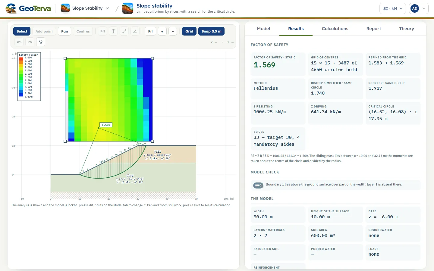
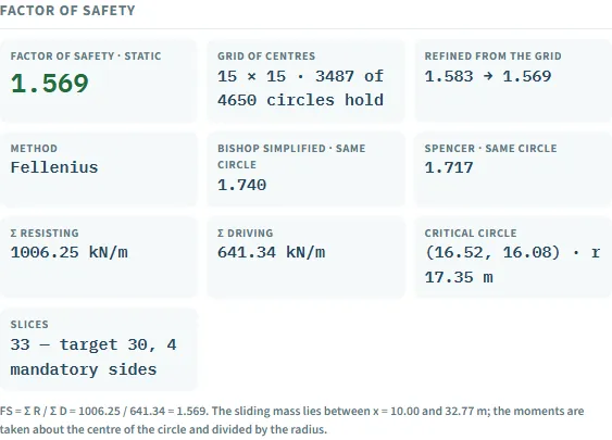
The three values are for the same circle, the critical circle of the Fellenius run (centre 16.52, 16.08, r 17.35 m): the Results tab lists the other two methods for it. When you choose Bishop or Spencer the grid is searched with that method, so the critical circle and its factor change: the example gives 1.720 (Bishop) and 1.699 (Spencer). A pseudo-static case uses the governing (lower) factor in the search. Where Spencer has no solution on a circle, or a tension between slices above the tolerance, the circle is left out and the Results tab says how many.
Analyze and read the results
Press Analyze. The bar reads Analysing… while the circles run (about a second for the example; a model with geogrids took about 15 s). The module switches to Results, a short message appears at the bottom of the window (for the example “FS = 1.569 — the critical of 3487 circles”), the bar reads the factor and the circle, and the model is locked; Edit inputs in the bar unlocks it. The bar turns warm when a factor is below 1 or when slice bases lost effective normal compression.
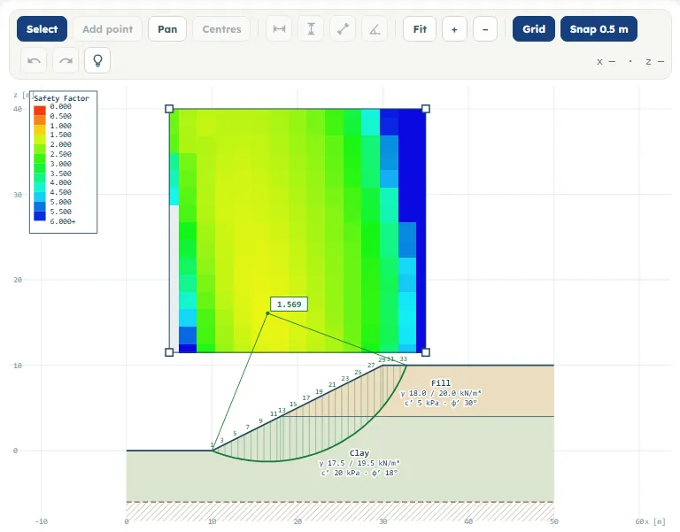
Factor of safety cards: static (and pseudo-static), the grid and how many of its circles hold (3487 of 4650 on the example), the refinement (1.583 → 1.569), the method, the other two methods on the same circle, Σ resisting, Σ driving (and the part of the resistance that is nails and geogrids, or the anchors taken off the driving side), the critical circle and the slices. Under the cards: Model check, The model (areas), Loads, Slices, and Soil at a point (type x and z, press Probe).
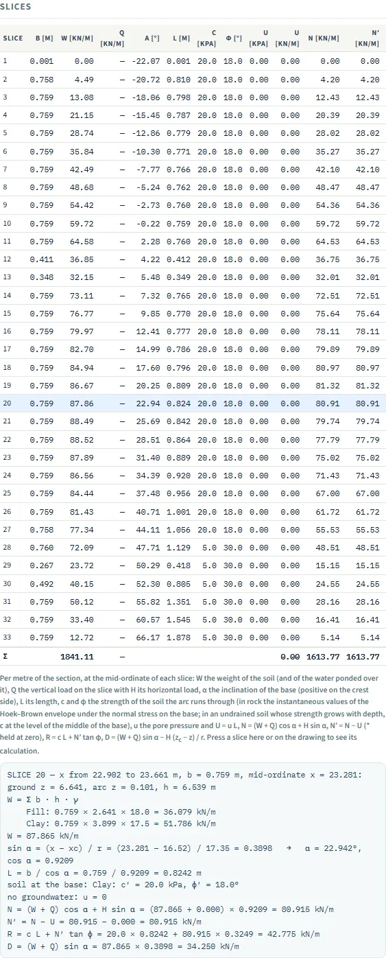
Press a slice, in the table or on the drawing, for its complete working: weight by soil, α, L, the strength at the base, pore pressure, N, N′, R and D, and for Spencer the forces between slices.
The drawing shows the critical circle, its slices with their numbers, and the colours of the centres: every centre of the grid coloured by its lowest factor (a legend gives the scale). A line joins the critical centre to the circle.
The Calculations tab, the report and the Theory tab
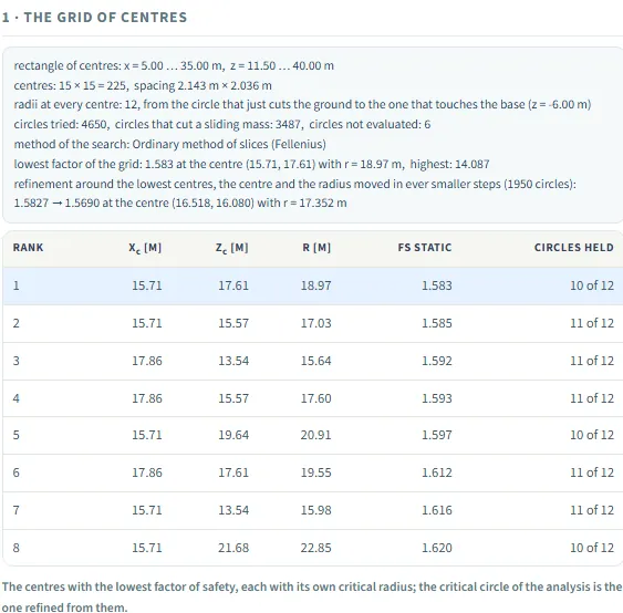
Calculations has five numbered sections: 1 · The grid of centres (the rectangle, circles tried and held, the lowest centres, the refinement; for a polyline 1 · The search for the slip surface), 2 · The critical circle (The critical surface for a polyline), 3 · The method, 4 · The slices, one by one and 5 · The factor of safety (all slices with the sums, the static and pseudo-static factors, the other methods on the same circle). When the model has reinforcement a section The reinforcement comes after the critical circle and the later ones move down by one, so the factor of safety is section 6.
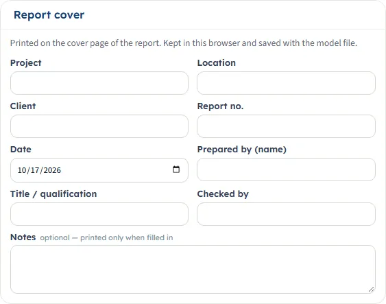
The Report tab has the cover (Project, Location, Client, Report no., Date, Prepared by, Title / qualification, Checked by, Notes), a preview, Save as PDF and Download Word (.docx). Without an analysis it is the model report; after it, a calculation report. For the example the parts are: Analysis summary, The model, Materials, Layers, Groundwater, Loads on the surface, Critical slip circle and slices, Factor of safety by the ordinary method of slices, Checks of the model. With reinforcement the parts Reinforcement and (for nails) Soil nails on the critical circle are added, and with an earthquake Pseudo-static earthquake; the part on the factor of safety is named after the method you chose. The analysis warnings are listed under the checks.
The Theory tab explains the method in 24 sections: the section and the strength of the soil, the factor of safety and the slices, water and loads, the three methods and how they compare, the earthquake, the tension crack, the search for the critical circle and for non-circular surfaces, the reinforcement (nails, anchors, geogrids), the rock criterion, the DXF section, a worked model, what the module assumes and its references.
Worked example: the module’s own example
Open the module and press Analyze: 10 m slope at 2H:1V, Fill (γ 18, c′ 5, φ′ 30) 4 m thick over Clay (γ 17.5, c′ 20, φ′ 18), no water, Fellenius, 30 slices target. The critical circle has its centre at (16.518, 16.080) and radius 17.352 m; the arc enters the ground at x = 9.999 m and leaves at 32.769 m. The module cuts 33 slices (four sides forced by the geometry at x = 10, 18, 28.973 and 30 m).
One slice by hand (slice 2, x from 10.000 to 10.758 m). The middle is x = 10.379 m: the ground is at z = 0.189 m and the arc at z = −0.149 m, so h = 0.338 m of Clay and W = 0.758 × 0.338 × 17.5 = 4.49 kN/m. sin α = (10.379 − 16.518) / 17.352 = −0.3538 (α = −20.72°), L = 0.758 / cos α = 0.810 m, N = W cos α = 4.20 kN/m, R = c′L + N tan φ′ = 20 × 0.810 + 4.20 × tan 18° = 17.57 kN/m, D = W sin α = −1.59 kN/m (this slice resists).
The same slices recomputed independently, outside the module, give 1.5690 (ordinary), 1.7401 (Bishop) and 1.7170 (Spencer, θ = 18.54°). With an earthquake (kh = 0.15 toward −x, kv = 0.05 downward) on the critical circle of that run (centre 16.719, 17.448, r 18.698 m) the independent values are 1.5756 / 1.7345 / 1.7139 static and 1.1379 / 1.2650 / 1.2502 pseudo-static, as the module gives.
Reinforcement by hand. A nail of the default row has bond qu π Dh = 100 × π × 0.1 = 31.42 kN/m. Nail N1 on the critical circle of its run has Lb = 2.03 m behind the surface, so pull-out behind = 31.42 × 2.03 ≈ 63.8 kN (the module works with Lb = 2.028 m and gives 63.7 kN, governing, below the bar tension 200 kN and the pull-out in front plus head); per metre 63.7 / 1.5 = 42.48 kN/m. The anchor A1 (bond 150 π 0.15 = 70.69 kN/m) has Lb = 2.89 m: 70.69 × 2.89 = 204 kN, less than P = 300 and Tt = 500, so the root pull-out governs: 204.0 kN, 81.59 kN/m.
How each input changes the answer
Each row changes one thing in the example (Fellenius, 15 × 15 × 12 grid, no water) and re-runs the module. The factor is that of the critical circle found for that model. Unless a row says otherwise the soils are Fill (γ 18 / 20 kN/m³, c′ 5 kPa, φ′ 30°) and Clay (γ 17.5 / 19.5 kN/m³, c′ 20 kPa, φ′ 18°), and a water line is level across the whole width.
| Change what it replaces | FS static circle: centre (x, z), r |
|---|---|
| The examplereference | 1.569(16.52, 16.08) 17.35 |
| Bishopmethod | 1.720(15.50, 19.64) 20.40 |
| Spencermethod | 1.699(15.51, 18.88) 19.67 |
| Clay c′ 10 kPawas 20 | 1.241(15.88, 15.59) 16.67 |
| Clay c′ 30 kPathe circle moves into the Fill | 1.774(19.06, 19.52) 15.51 |
| Clay φ′ 12°was 18° | 1.296(17.54, 14.63) 16.70 |
| Clay φ′ 24°again within the Fill | 1.774(19.06, 19.52) 15.51 |
| Clay γ 20.5 / 22.5was 17.5 / 19.5 | 1.579(16.20, 16.08) 17.23 |
| Fill c′ 0, φ′ 25°weaker fill | 0.944(15.63, 22.70) 18.23 |
| Slope 3H:1V (G3 at x = 40)flatter | 1.995(21.37, 21.38) 24.84 |
| Slope 1H:1V (G3 at x = 20)steeper | 1.087(10.46, 12.26) 12.27 |
| Water at z = 5 m, level (clamped on the lower ground) | 1.144(17.05, 11.28) 15.64 |
| Water at z = 10 m (the crest), clamped | 0.894(21.56, 14.55) 10.55 |
| Water at z = 5 m, ponded on the slopeits weight and pressure act on the face | 1.474(18.54, 12.82) 15.41 |
| Water at z = 10 m (the crest), ponded | 1.715(22.16, 13.54) 9.53 |
| Clay ru 0.3 | 1.272(17.66, 13.15) 15.97 |
| Clay undrained cu 50 kPa | 1.533(20.03, 15.57) 21.57 |
| Strip load 20 kPa on the crestbeyond the mass: no effect | 1.569(16.52, 16.08) 17.35 |
| Strip load 50 kPa on the crest | 1.511(18.46, 20.55) 22.40 |
| Tension crack 2 m, dry | 1.584(16.70, 15.59) 16.97 |
| Nails: row of 3 (defaults) | 1.601(17.42, 15.71) 17.67 |
| One anchor (defaults) | 1.668(17.59, 14.54) 17.44 |
| Geogrids: row of 3 (defaults)about 15 s to run | 1.597(17.09, 15.68) 17.26 |
| Base at z = −3 m, or −12 m | 1.569the circle does not reach it |
| Slices 10 / 30 / 100 | 1.558 / 1.569 / 1.571 |
- Strength of the Clay stops mattering once the critical circle can stay in the Fill: c′ 30 kPa and φ′ 24° give the same 1.774.
- Ponded water presses on the ground it stands on and its weight acts there, so the same line at z = 5 m gives 1.474 ponded against 1.144 held at the ground surface; on the ponded circle 4 slice bases lose effective normal compression and the module says so. The same two cases by Bishop give 1.827 and 1.429, by Spencer 1.811 and 1.425.
- Earthquake (kh 0.15, critical direction): 1.579 static and 1.147 pseudo-static; with kv 0.075: 1.575 and 1.134.
- Reinforcement raises the factor only where a circle crosses it and its tip lies behind the surface: in the nail run, N3 carries nothing on that circle.
- The result depends on the search: the factor is the lowest of the circles tried, so a coarser grid or fewer slices moves it slightly.
Messages
Model check (button, and on the Results tab) lists ERROR, WARNING and INFO lines. A model with an ERROR is not analysed; pressing Analyze opens a window Analysis. Examples, quoted:
- “The model has 1 error — see Model check on the Results tab.” with “The base of the model must lie below the lowest point of the ground surface (now 2.00 m against 0.00 m).” (base z = 2).
- “Soil "Clay" has no strength: c′ = 0 and φ′ = 0.”
- “No slip circle of the grid of centres cuts a sliding mass out of the slope: move the rectangle of centres over the face of the slope.”
- “Boundary 1 lies above the ground surface over part of the width: layer 1 is absent there.” (INFO, in the example.)
- (a level water line at z = 12 m) “The water line stands above the ground surface between x = 0.00 and 50.00 m (300.00 m²); it is held at the ground surface there and no water stands on the slope — the choice "Where the line stands above the ground" in the Groundwater section decides.” (WARNING.)
- “Static: Loss of effective normal compression on 6 slice bases: the pore force exceeds the normal force there and N′ has been taken as zero, the usual practice of the ordinary method of slices.” followed by a request to review the groundwater and the slip surface; the slices are marked orange.
- “N3 carries nothing — tip inside the mass” in the reinforcement table.
- Files: “Not a model file: no ground surface found in the file”; with no quick save chosen: “Choose a saved model first.”; a DXF without lines: “No lines were found in the DXF file (LWPOLYLINE, POLYLINE or LINE in the ENTITIES section).”
Spencer. On a circle where the forces and the moments do not balance at any angle of the forces between the slices, or where the forces between the slices come out as a tension above 2 % of the largest one, the circle is not a candidate. The Calculations tab counts them in the grid line: on a steep face (the ground rising 15.2 m over 5 m, c′ 43 kPa, φ′ 7° in both soils, a 12 × 12 grid) it reads “circles tried: 2550, circles that cut a sliding mass: 583, passed over because their equations have no solution: 215, left out because the Spencer solution is not admissible (a tension between the slices above the tolerance): 945”. With the ordinary method the same line reads “circles not evaluated: N” for a circle that could not be evaluated. Warnings of a Spencer solution look like these (each is followed by a request to review the groundwater and the slip surface, and the slices concerned are marked orange): “The normal force between the slices is negative — a tension — at 1 of the sides (the lowest -13.4 kN/m, 2.1% of the largest interslice force, above the tolerance of 2%): the solution is not admissible there.”, “On 10 slice bases the denominator of ΔE falls under 0.2 FS / cos θ and has been held there: the base is steeply inclined against the sliding.”, “The angle of the forces between the slices is 56.2°, outside the range of an ordinary solution.” and “Loss of effective normal compression on 1 slice base: the equilibrium gives a negative N′ there and the friction has been left out, the cohesion kept.” When every circle that cuts a mass is left out for this reason the module asks you to change the model or the rectangle of centres.
Good practice
- Look at the colours of the centres: the lowest centre should lie inside the rectangle, not on its edge (the Results tab warns when it still does after the grid widened).
- Start with the ordinary method for a quick look and use Bishop or Spencer for the factor you report; compare the three on the same circle.
- Give γsat and the water line for a slope below the water table, and choose what happens where the line stands above the ground.
- Use Model check before Analyze, and read every WARNING after it.
- Choose kh and kv yourself for the earthquake and keep the critical direction unless you know the direction.
- Save the model to a file as well: the browser keeps only the last model.
Frequently asked questions
How is the factor of safety of a slope calculated?
By the method of slices: the mass above a slip surface is cut into vertical slices, and the factor is the resisting moment divided by the driving moment (ordinary and Bishop) or the value at which forces and moments both balance (Spencer). The module does this for every circle of a grid and keeps the lowest.
Which method should I use?
On the example the same circle gives 1.569 (ordinary), 1.740 (Bishop) and 1.717 (Spencer). Spencer satisfies forces and moments and is the one used for non-circular surfaces.
Why is the critical circle on the edge of the rectangle?
The module widens the grid on that side by itself; if the lowest centre still stands on the edge the Results tab says so and you enlarge the rectangle.
Does the module keep my model?
Yes. Every change is kept by the browser and the page opens on it; the analysed state is not kept. Save to a file or Quick Save to keep versions.
Can I work in US units?
No: the module works in m, kN/m³, kPa and degrees and holds the unit selector on SI · kN.
How do I add an earthquake?
Switch on Pseudo-static analysis in Earthquake and give kh and kv; both factors are then shown.
Why does an anchor reduce the driving side?
An anchor is stressed before the mass moves, so its force is taken from the driving moment; nails and geogrids work as the mass moves and add to the resistance.
What does a nail "carry nothing" mean?
On that circle its tip lies inside the sliding mass or its head outside it, so it does not cross the slip surface.
Can I analyse a non-circular surface?
Yes: choose Not circular in Slip surfaces. The search starts from the surface drawn, the critical circle and each boundary, and Spencer analyses the result.
Can I import a drawing?
Yes, a DXF with the layers EXTERNAL, MATERIAL, WATER TABLE (a space or an underscore between the words), NAIL, ANCHOR and GEOGRID, with Import DXF… in Model data. The button DXF format & examples… beside it explains how to draw the section.
Is there an example DXF file to start from?
Yes: DXF format & examples… in Model data has three to download: a slope with a water table, a cut held by soil nails and a ground anchor, and an embankment with geogrids. Each opens in any CAD program and is read by Import DXF… as it is.
Why can I not edit after Analyze?
The model is locked while results are shown; press Edit inputs.
How can I check a result by hand?
Open the Calculations tab and the section The slices, one by one: each slice has its working. On slice 2 of the example, W = 0.758 × 0.338 × 17.5 = 4.49 kN/m and R = 20 × 0.810 + 4.20 × tan 18° = 17.57 kN/m.