

What the module calculates
SPT triggering checks whether liquefaction is triggered in a site with several boreholes. For every standard penetration test below the groundwater table it corrects the blow count, works out the cyclic stress ratio CSR (the demand of the earthquake) and the cyclic resistance ratio CRR (what the soil can carry), and gives the factor of safety:
FS below 1.0 is triggered; FS from 1.0 up to the required value FSreq is marginal; above it the result is OK. The method is Idriss & Boulanger (2014); the magnitude Mw and the peak ground acceleration amax are your inputs.
What you get
- The corrected blow counts, CSR, CRR and FS of every test, with a step-by-step calculation of each one.
- The triggered and marginal zones of every borehole, their thickness, and the minimum FS with its depth.
- Colour-band sections between the boreholes, or colour columns when no section is defined, and a project summary with every borehole side by side.
- An Excel template (one sheet per borehole) to fill in and import, model files, and a Word or PDF summary report.
What belongs elsewhere
- Tests in clay-like soil are listed but not evaluated; the module reminds you to check those layers for cyclic softening separately. Consequences of liquefaction (settlement, lateral spreading, loss of bearing capacity) are outside this module.
- Cone penetration data have their own module: CPT triggering.
Before you start: what you need
| What | Source | Notes |
|---|---|---|
| Each borehole: name, groundwater depth, ground elevation | Boring logs, site survey | The groundwater depth is measured from the ground surface of that borehole. |
| Soil layers of each borehole | Boring logs, laboratory tests | USCS symbol, description, unit weight γ and saturated unit weight γsat , plasticity index PI (blank for non-plastic) and fines content FC. The first layer starts at the ground surface and each layer starts where the one above ends. |
| The SPT tests | Field blow counts | Depth and the raw field blow count N30 (last 30 cm, no correction); a laboratory fines content for a test is optional. |
| The design earthquake | Your design | Peak ground acceleration amax in g (site effects included) and moment magnitude Mw. |
| The test equipment | Boring report | Hammer energy ratio ER, borehole diameter, sampler type, rod stick-up above the ground. |
| For sections: distances along the line | Site plan | The distance of each borehole along each section line, in metres (or the unit of the page). |
Quick start in eight steps
- Open the module and choose the units
Open SPT triggering from the Liquefaction family. Pick SI · kN, SI · tf or US in the header.
- Enter the boreholes
In Boreholes, Soil layers and SPT tests, enter each borehole, or fill the Excel template and use Import Excel….
- Define the sections
In Sections, name a line through some of the boreholes and give the distance of each along it. Without a section the Contours view shows colour columns.
- Enter the earthquake
In Earthquake, type amax and Mw.
- Set the corrections and the settings
In SPT corrections give the hammer energy ratio, borehole diameter, sampler and stick-up; in Analysis Settings the required factor of safety, the clay-like limit and the deepest test.
- Press Analyze
Press Analyze. The bar reads Analysed, the inputs lock and the Contours view opens. A Warnings window opens when the run carries warnings.
- Read the answer
Look at the colour bands, the Borehole and Project summary views and the Results tab; open Calculations for any test.
- Take the report
In Report fill in the cover, then save a PDF or download a Word file.
The screen: three views, five tabs
The layout is the shared GeoTerva one, described in the workspace guide. The drawing has three views, chosen above it; the right-hand panel has the tabs Model, Results, Calculations, Report and Theory.
- Borehole shows one borehole: its soil log with the groundwater level, the N30 and (N1)60cs points, the CSR curve against the CRR points, and the factor of safety against depth with the triggered and marginal zones tinted. Grey hatched bands are not evaluated (above the groundwater, clay-like, or deeper than the limit). Choose the borehole with the buttons above the drawing. Layers chips (N₃₀ field, (N₁)₆₀cs, Result zones, FS values) hide or show parts of the drawing; the analysis always uses every test.
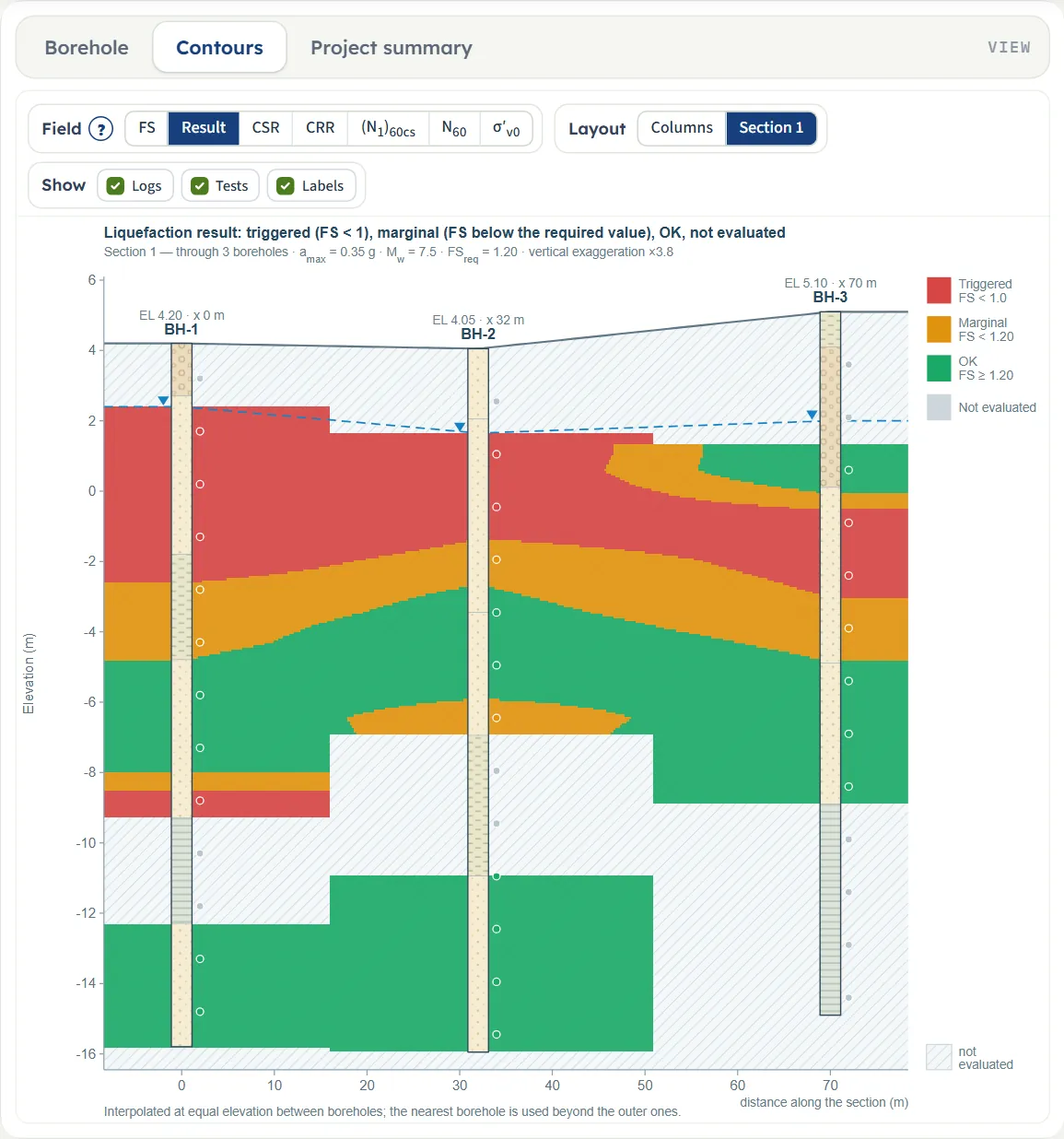
- Contours draws colour bands of a chosen Field over the section between the boreholes. It is the view that opens after Analyze.
- Project summary plots FS against depth for all boreholes, and a fence of every borehole side by side (soil on the left half, result on the right half) with its minimum FS. One chip per borehole switches its curve.
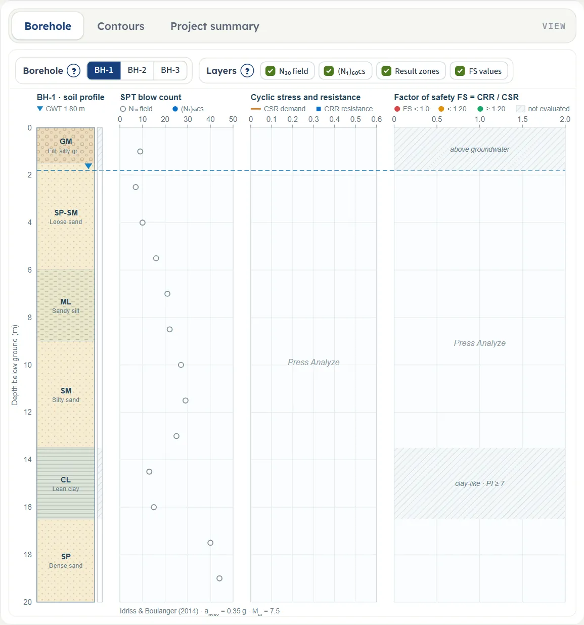
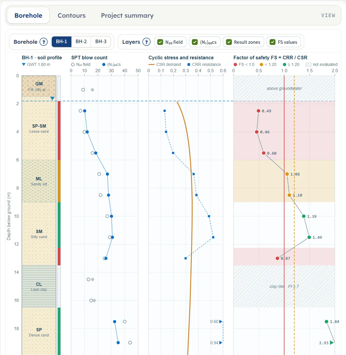
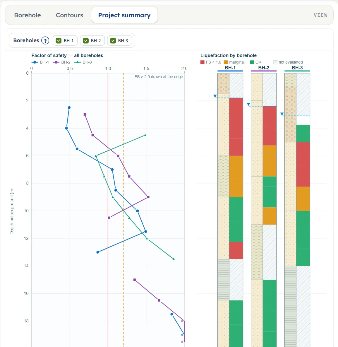
The Contours controls
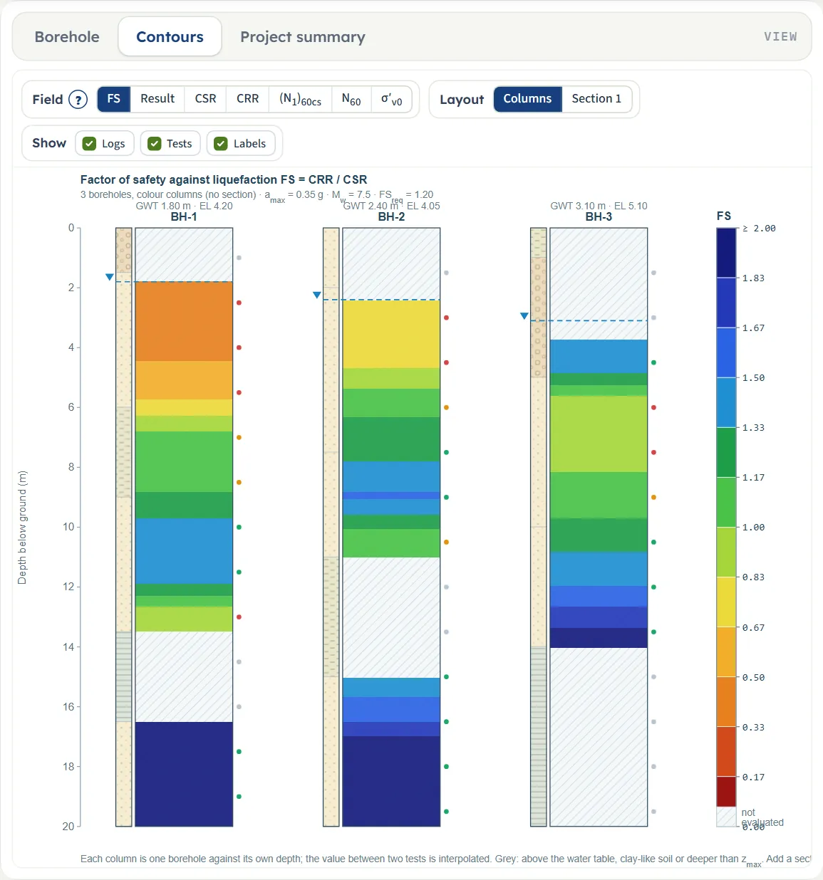
- Field: FS (the factor of safety), Result (triggered, marginal, OK as three colours), CSR, CRR, (N₁)₆₀cs, N₆₀ and σ′v0 (the initial effective vertical stress). One legend serves all panels.
- Layout: Columns (every borehole as its own colour column against its own depth, no interpolation), one button per section, and All when there are two or three sections (one panel under the other).
- Show: Logs (the soil strip of each borehole), Tests (a dot at every test, coloured by result) and Labels.
Between two boreholes the field is interpolated linearly at equal elevation; beyond the outer boreholes the nearest one is used. Grey is not evaluated. The title line states the vertical exaggeration of the section.
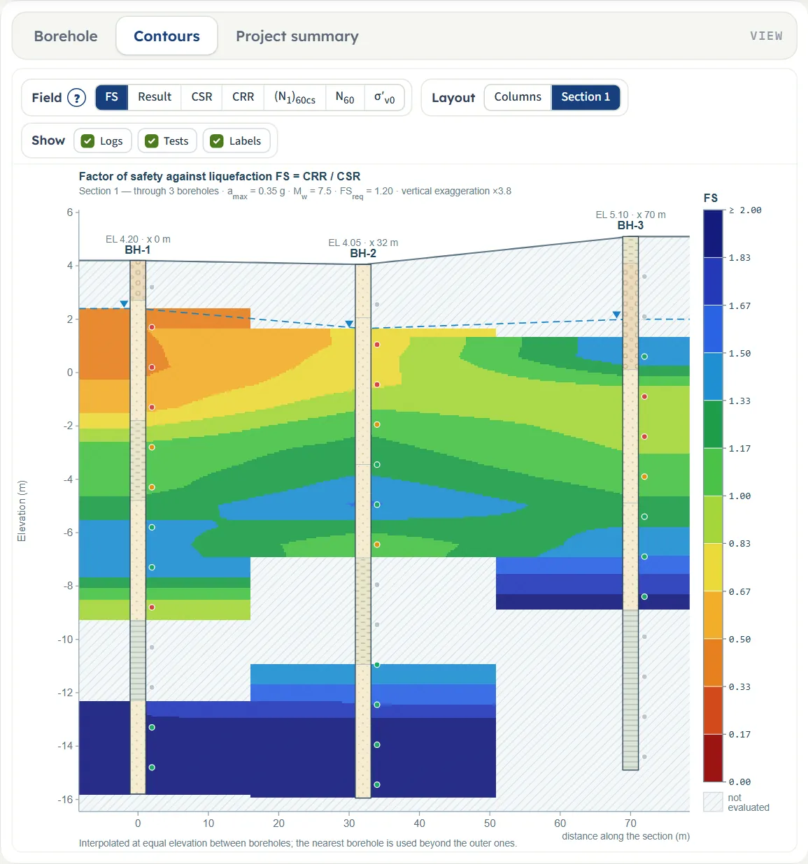
What stays after a reload
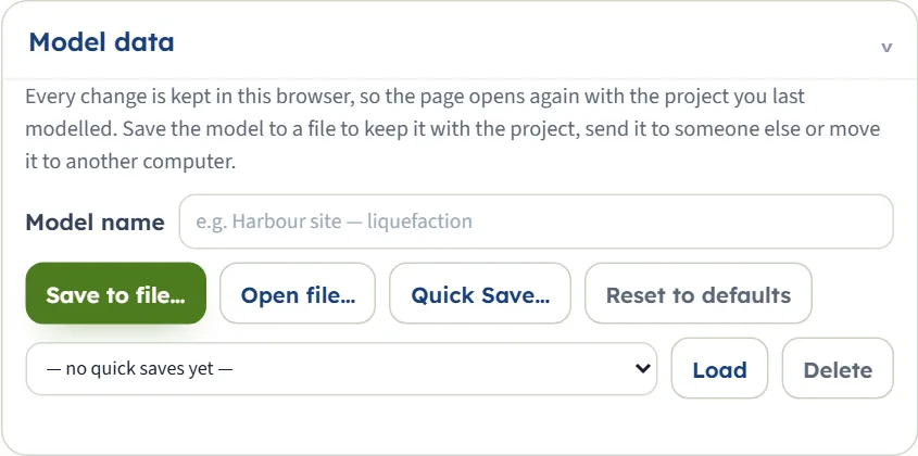
Unlike some other modules, this one keeps your work. Every change is stored in the browser, and the page opens with the project you last worked on (also when it was analysed: it opens analysed). The store message names the time. Save to file… writes the model to a .gtrv file you can send or move, Open file… reads one, Quick Save… keeps named versions in the browser list with Load and Delete, and Reset to defaults returns to the example. The model name box names the file and the Excel template.
Entering the model, section by section
The Model tab is a column of sections. Model data stays open on its own; the others form an accordion: opening one closes the previous one, and Next and Back walk through them. The inputs lock after Analyze (Edit inputs unlocks them and clears the results). A box you leave empty goes back to its last value; a value the module cannot use is reported when you press Analyze.
Model data and Excel input
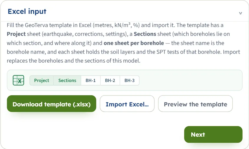
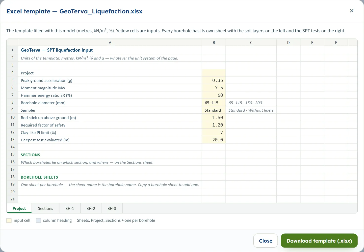
The Excel input section has Download template (.xlsx) (the template filled with the current model, named after the model), Import Excel… and Preview the template. The template has a Project sheet (earthquake, corrections, settings), a Sections sheet (which borehole lies on which section, and where) and one sheet per borehole, whose name is the borehole name, with the soil layers on the left and the SPT tests on the right. It always holds metres, kN/m³, % and g, whatever the unit system of the page.
Boreholes
A project holds any number of boreholes. Choose one with the buttons (each shows its number of tests and, after Analyze, its result); + Add borehole, Duplicate and Delete borehole (the project keeps at least one) change the list.
A new borehole starts with zw = 2 m, EL = 0, one layer of silty sand to 10 m and tests at 1.5, 3 and 4.5 m (N30 10, 12, 14).
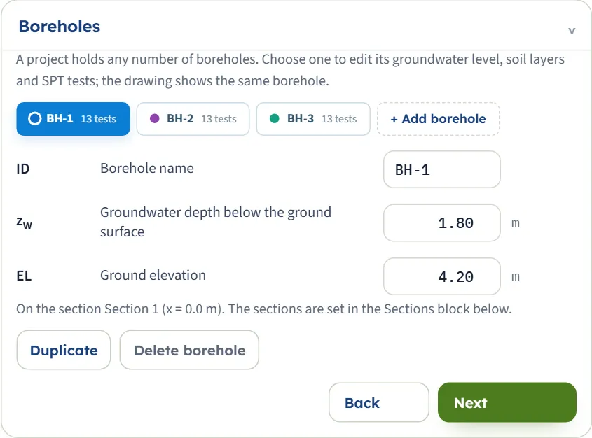
| Field | Default | Notes |
|---|---|---|
| Borehole name ID | BH-1 | Up to 24 characters; a name already used is not accepted. |
| Groundwater depth zw | 1.80 m | Below the ground surface of this borehole. Also 2.40 m (BH-2) and 3.10 m (BH-3). |
| Ground elevation EL | 4.20 m | Used to place the borehole in a section. 4.05 m and 5.10 m for BH-2 and BH-3. |
Sections
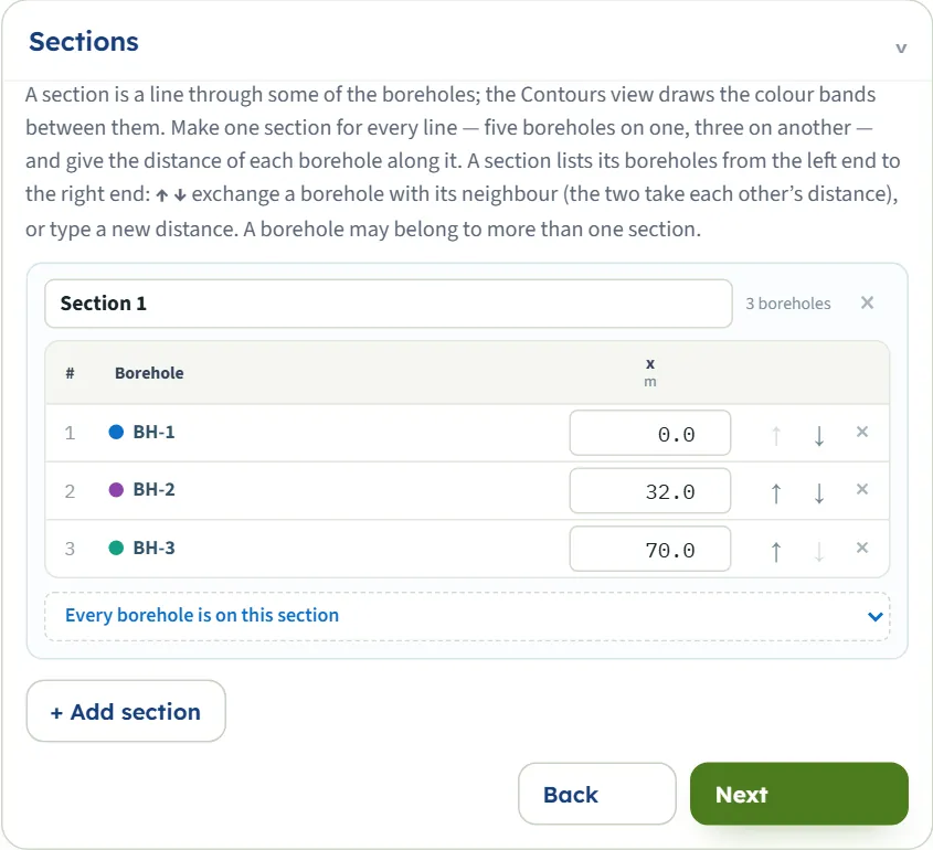
A section is a line through some of the boreholes; the Contours view draws the colour bands between them. + Add section adds one, named “Section n”. In each section the boreholes are listed from the left end to the right end with their distance along the line. ↑ ↓ exchange a borehole with its neighbour (they take each other’s distance), the distance box accepts a new value, × takes the borehole out, and the list under the table adds one. A borehole may belong to several sections. The example has one section: BH-1 at 0 m, BH-2 at 32 m, BH-3 at 70 m.
Soil layers
From the ground surface down; To is the only depth you type, the next layer starts there. The PI box decides the screening and FC is the fines content used for the tests of the layer that have no laboratory value. + Add layer adds a 2 m layer of silty sand (γ 18, γsat 19.5, FC 20) below the last one; × deletes a layer (the last layer cannot be deleted).
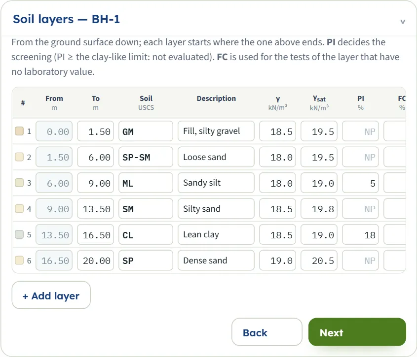
| Field | Default | Notes |
|---|---|---|
| From, To | 0.00 – 1.50 … | m; the profile of BH-1 ends at 20 m. |
| Soil (USCS), Description | GM, Fill, silty gravel … | A symbol from the list or your own; when PI is blank, CL, CH, OL, OH and PT mean clay-like. |
| γ, γsat | 18.5 / 19.5 kN/m³ … | γ is used above the groundwater table and γsat below it. |
| PI | blank = NP | Percent; PI at or above the clay-like limit: not evaluated. |
| FC | 20 % | Percent. |
SPT tests
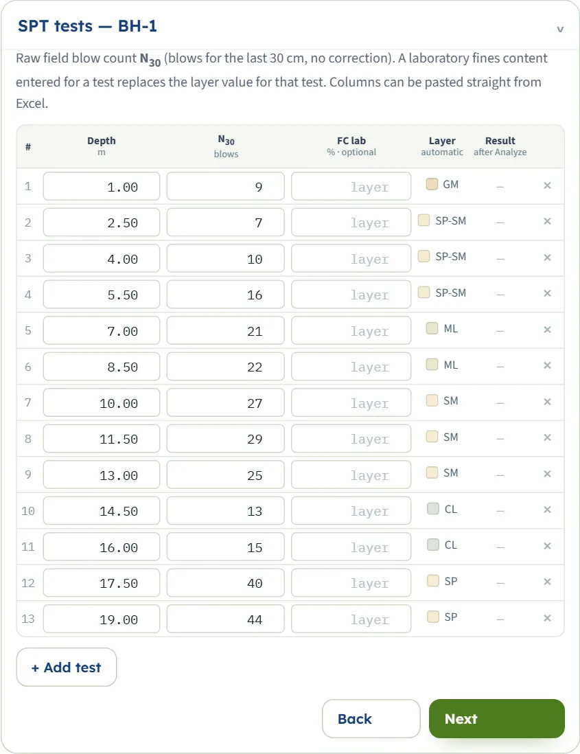
Depth, the raw field blow count N30 , and an optional laboratory FC lab that replaces the layer value for that test. The Layer column names the layer found at the depth, and the Result column shows the FS after Analyze (a pill: triggered, marginal, OK) or N/E for not evaluated. + Add test adds a test 1.5 m below the deepest with N30 = 10. Columns can be pasted straight from Excel.
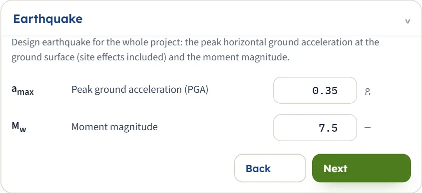
Earthquake
The earthquake is one for the whole project.
| Field | Default | Notes |
|---|---|---|
| Peak ground acceleration amax | 0.35 g | At the ground surface, site effects included. Must be above zero. |
| Moment magnitude Mw | 7.5 | The box is set for 4 to 9.5. Must be above zero. |
SPT corrections
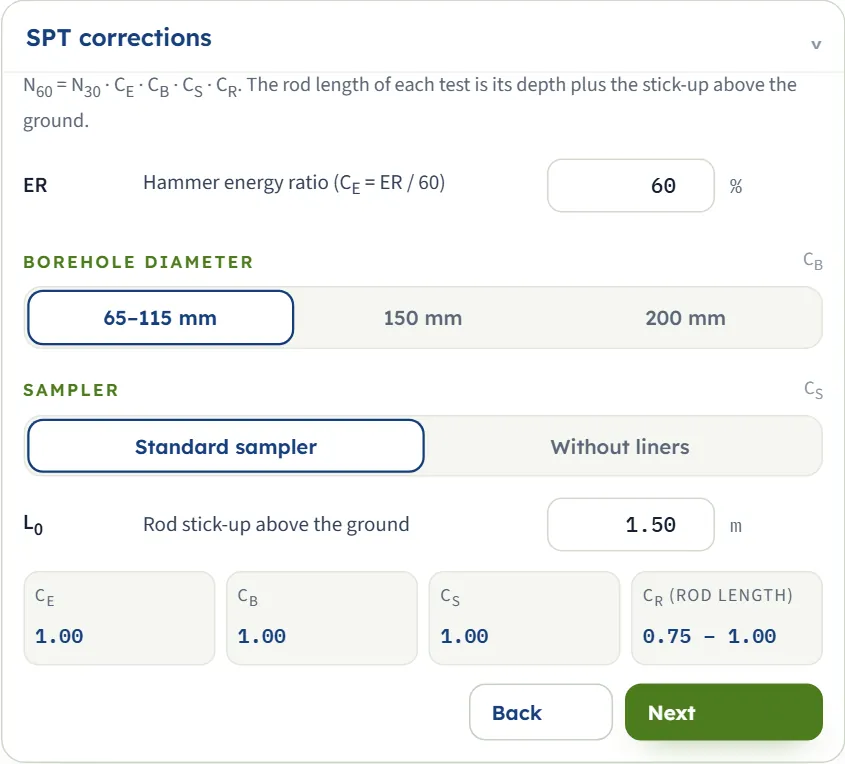
N60 = N30 · CE · CB · CS · CR. The rod length of a test is its depth plus the stick-up.
Read-only boxes show the CE, CB and CS in use.
| Field | Default | Notes |
|---|---|---|
| Hammer energy ratio ER | 60 % | CE = ER / 60. |
| Borehole diameter CB | 65–115 mm | Buttons: 65–115 mm (1.00), 150 mm (1.05), 200 mm (1.15). |
| Sampler CS | Standard sampler | Standard sampler (1.00) or Without liners (1.20). |
| Rod stick-up L0 | 1.50 m | Above the ground; CR follows the rod length: 0.75 below 3 m, 0.80 below 4 m, 0.85 below 6 m, 0.95 below 10 m, 1.00 beyond. |
Analysis Settings
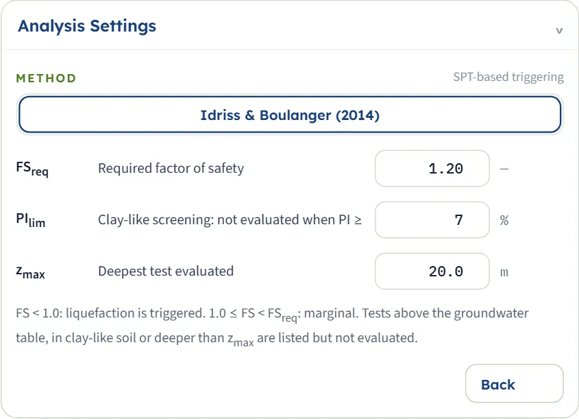
The method button shows Idriss & Boulanger (2014); it is the one method.
| Field | Default | Notes |
|---|---|---|
| Required factor of safety FSreq | 1.20 | Below it (and from 1.0) a test is marginal. |
| Clay-like screening PIlim | 7 % | Not evaluated when PI is at or above it. |
| Deepest test zmax | 20 m | Deeper tests are listed but not evaluated. |
The Excel template, step by step
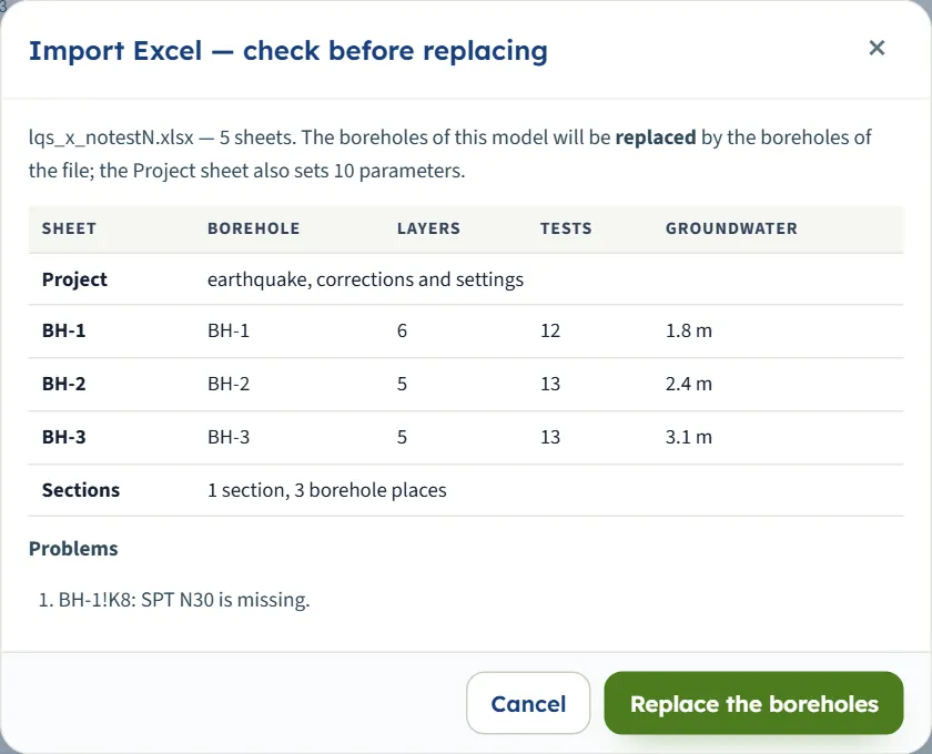
Use Preview the template to see the sheets in a window, or download it. Yellow cells are inputs. On import the module shows a window, Import Excel — check before replacing, listing each sheet (borehole name, layers, tests, groundwater), the sections found and any problems; Replace the boreholes replaces the boreholes and the sections of the model (and the project settings the Project sheet carries). Import is not offered while results are shown: Edit inputs first.
The method and its options
There is one method, Idriss & Boulanger (2014). What you can choose is how the tests are corrected and screened:
- Equipment corrections — ER, borehole diameter, sampler and stick-up. They scale N60 : a higher energy ratio or a larger factor raises N60 and the resistance.
- Fines — the fines content of the layer (or the laboratory value of the test) adds Δ(N1)60 to the corrected count, so a silty sand is stronger than a clean one at the same blow count.
- Screening — tests above the groundwater table, deeper than zmax or in clay-like soil (PI at or above PIlim ; CL, CH, OL, OH, PT when PI is blank) are listed but not evaluated.
- Required factor of safety — it only separates marginal from OK; the triggered limit is always 1.0.
Each evaluated test stands for its layer from halfway to the neighbouring test above to halfway to the one below; neighbouring intervals with the same result merge into zones.
Analyze and read the results
Press Analyze. The bar counts the boreholes (“Analysing… BH-1 (1 / 3)”) and then reads Analysed — 3 boreholes, 39 tests, adding the number of warnings. The view switches to Contours, a short message says the colour bands show the selected field, and, when there are warnings, the Warnings window opens by itself. The module stays on the Model tab: open Results.

Results tab
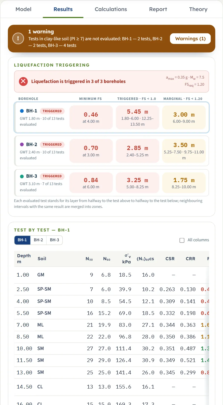
At the top a line says Liquefaction is triggered in 3 of 3 boreholes (or “not triggered in any borehole”), with amax , Mw and FSreq . One row per borehole follows: its result chip, the groundwater depth, how many tests were evaluated, the minimum FS with its depth, the triggered thickness with the zones, and the marginal thickness with the zones. Clicking a row selects the borehole.
| Borehole | Triggered | Marginal |
|---|---|---|
| BH-1 minimum FS 0.46 at 4.00 m | 5.45 m 1.80–6.00, 12.25–13.50 m | 3.00 m 6.00–9.00 m |
| BH-2 minimum FS 0.70 at 3.00 m | 2.85 m 2.40–5.25 m | 3.50 m 5.25–7.50, 9.75–11.00 m |
| BH-3 minimum FS 0.84 at 6.00 m | 3.25 m 5.00–8.25 m | 1.75 m 8.25–10.00 m |
Test by test
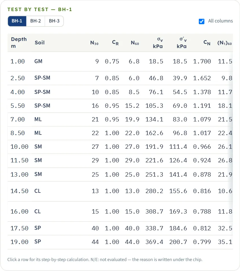
Below, a table lists every test of the chosen borehole: depth, soil, N30 , N60 , σ′v, (N1)60cs , CSR, CRR, FS and the result chip. All columns adds CR, σv, CN, (N1)60 , FC, Δ(N1)60 , rd, CRR7.5 , MSF and Kσ. A test that is not evaluated shows N/E with the reason (above groundwater, clay-like (PI ≥ 7), deeper than zmax ). Click a row for its calculation.
Warnings
The Warnings window lists the warnings and the assumptions of the analysis. The warnings the module writes are:
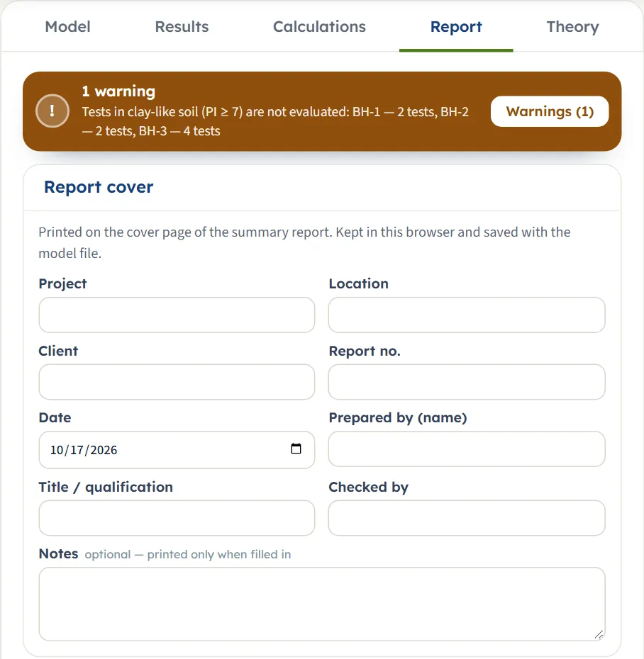
- “Tests in clay-like soil (PI ≥ 7) are not evaluated: BH-1 — 2 tests, BH-2 — 2 tests, BH-3 — 4 tests. Check these layers for cyclic softening separately.” (the example)
- “(N₁)₆₀cs ≥ 37, taken at the upper limit of the CRR curve: BH-1 at 10.00, 11.50, 17.50, 19.00 m; BH-2 at 7.50, 9.00, 15.00, 16.50, 18.00, 19.50 m; BH-3 at 10.50, 12.00, 13.50 m.” (the example with ER = 80 %: it appears when a corrected count reaches the end of the CRR curve)
- “No fines content given for BH-1 layer 2 — FC = 0 % is used.”
- “No test evaluated in BH-1 (all above the water table, clay-like or deeper than the deepest test).” (the module writes the last words with a z and a subscript max)
The bar turns amber and the Results and Report tabs carry the same warning bar.
The Calculations tab, the report and the Theory tab
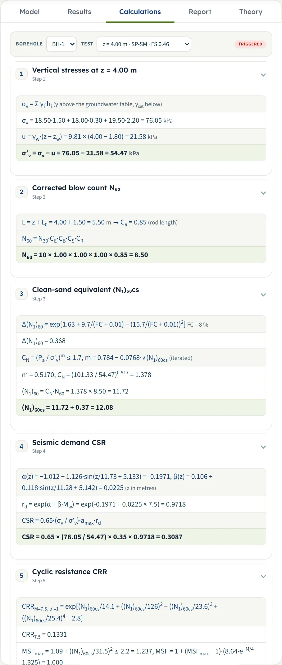
The Calculations tab writes out one test. Choose the borehole and the test in the two lists (or click a row or a mark), and six steps follow with your numbers: 1 vertical stresses, 2 corrected blow count N60 , 3 clean-sand equivalent (N1)60cs (with CN iterated on its exponent), 4 seismic demand CSR, 5 cyclic resistance CRR (with MSF and Kσ), 6 factor of safety. A test that is not evaluated stops after step 3 with the reason. Each step opens and closes.
The report
In Report fill in the cover (project, location, client, report number, date, prepared by, title / qualification, checked by, optional notes); it is kept in the browser and saved with the model file. After Analyze Save as PDF (opens a print window: choose “Save as PDF” as the printer) and Download Word (.docx) are available, and the preview shows the report. Its parts: 1 Introduction and scope, 2 Boreholes and soil profiles (borehole table, sections, layers of every borehole), 3 Earthquake, SPT corrections and settings, 4 Results by borehole (with the contour figure and the project figure), 5 Test by test (a table and a figure for every borehole), 6 Warnings (only when the run has warnings) and 7 Summary.
The Theory tab has fourteen sections: Scope, Screening of the tests, Stresses, SPT corrections, Overburden correction, Fines content, Cyclic stress ratio, Cyclic resistance ratio, Magnitude scaling factor, Overburden factor, Factor of safety, Zones and thickness, References, Colour-band section. Its Scope section names the same method as Boulanger & Idriss (2014).
Worked example: BH-1 at 4.00 m
The default example, test at 4.00 m in BH-1 (SP-SM, FC 8 %, N30 = 10, groundwater at 1.80 m, amax = 0.35 g, Mw = 7.5, ER 60 %, stick-up 1.50 m). A separate Python calculation from the formulas the module states gives the same numbers.
- Stresses: σv = 18.5·1.5 + 18.0·0.3 + 19.5·2.2 = 76.05 kPa; the pore pressure below the groundwater table u = 9.81 × (4.00 − 1.80) = 21.58 kPa, so σ′v = 76.05 − 21.58 = 54.47 kPa.
- Rod length 4.00 + 1.50 = 5.50 m, CR = 0.85; N60 = 10 × 0.85 = 8.50.
- Δ(N1)60 = 0.368 (FC 8 %). By iteration m = 0.5170, CN = (101.33 / 54.47)0.517 = 1.378, (N1)60 = 11.72, (N1)60cs = 12.08.
- rd = exp(−0.1971 + 0.0225 × 7.5) = 0.9718; CSR = 0.65 × (76.05 / 54.47) × 0.35 × 0.9718 = 0.3087.
- CRR7.5 = 0.1331; MSF = 1.000 (Mw = 7.5); Kσ = 1.062; CRR = 0.1331 × 1.000 × 1.062 = 0.1413.
- FS = 0.1413 / 0.3087 = 0.46: below 1.0, triggered.
For the test at 2.50 m the module gives CSR = 0.263, CRR = 0.130 and FS = 0.49.
The same project in US units
Switch to US after Analyze: nothing is run again. BH-1 now reads groundwater 5.91 ft, the minimum FS 0.46 at 13.12 ft, the triggered zones 5.91–19.69 and 40.19–44.29 ft (17.88 ft) and the test table σ′v in ksf; the calculation shows σ′v = 1.14 ksf at 13.12 ft with CN = (2.12 / 1.14)0.517 = 1.378. The stick-up box shows 4.92 ft. FS is the same 0.46.
The same project in SI · tf
In SI · tf the stresses are in t/m²: σv = 7.75 and σ′v = 5.55 t/m² at 4.00 m, with CN = (10.33 / 5.55)0.517 = 1.378 (54.47 kPa ÷ 9.80665 = 5.55). Depths and zones stay in metres.
How each input changes the answer
Each row changes one thing in the example and runs the module again (typing into the boxes). The first table gives the test at 2.50 m of BH-1 (SP-SM, FC 8 %, N30 = 7, γsat = 19.5 kN/m³); the example gives CSR 0.263, CRR 0.130, FS 0.49.
| Change | CSR / CRR | FS |
|---|---|---|
| The example | 0.263 / 0.130 | 0.49 |
| amax = 0.25 g Lower demand; BH-1 triggered thickness 4.20 m | 0.188 / 0.130 | 0.69 |
| amax = 0.45 g Higher demand; thickness 8.45 m | 0.338 / 0.130 | 0.38 |
| Mw = 6.5 Smaller earthquake: CRR rises through the magnitude factor | 0.260 / 0.139 | 0.54 |
| Mw = 8.0 Larger earthquake: CRR falls | 0.265 / 0.126 | 0.48 |
| ER = 80 % N60 7.93; this run adds the warning for (N1)60cs ≥ 37 | 0.263 / 0.154 | 0.59 |
| ER = 45 % N60 4.46; thickness 15.20 m | 0.263 / 0.112 | 0.43 |
| Borehole 200 mm (CB 1.15) | 0.263 / 0.141 | 0.53 |
| Sampler without liners (CS 1.20) | 0.263 / 0.144 | 0.55 |
| Stick-up 0 CR 0.75 instead of 0.85 | 0.263 / 0.122 | 0.46 |
| Stick-up 3.0 m Same CR 0.85 here: no change at this test | 0.263 / 0.130 | 0.49 |
| BH-1 groundwater 1.0 m The test becomes the minimum of BH-1 | 0.324 / 0.134 | 0.41 |
| N30 = 12 at 2.50 m | 0.263 / 0.184 | 0.70 |
| N30 = 3 at 2.50 m | 0.263 / 0.090 | 0.34 |
| Layer 2 FC = 30 % | 0.263 / 0.169 | 0.64 |
| Layer 2 FC = 0 % | 0.263 / 0.127 | 0.48 |
| Layer 2 γsat = 21 kN/m³ Heavier layer: higher σ′v (40.98 kPa) | 0.262 / 0.128 | 0.49 |
| BH-1 groundwater 3.0 m The test lies above the groundwater: not evaluated | — | N/E |
The pattern: amax acts on CSR only; the magnitude, the corrections and the fines act on CRR only (the magnitude also on CSR through rd, slightly); the groundwater depth and the unit weight act on both through the stresses, and the blow count on CRR.
Settings change which tests count and how they are classed, not the FS of a test. Effect on the project (BH-1 triggered thickness, boreholes triggered / marginal-only of 3; the BH-1 minimum FS stays 0.46 in all five runs):
| Change | Triggered BH-1 | Boreholes |
|---|---|---|
| The example | 5.45 m | 3 / 0 |
| FSreq = 1.0 | 5.45 m | 3 / 0 |
| FSreq = 1.5 | 5.45 m | 3 / 0 |
| zmax = 10 m | 4.20 m | 3 / 0 |
| PIlim = 4 % | 5.45 m | 3 / 0 |
| PIlim = 20 % | 8.45 m | 3 / 0 |
In the second table the last column reads “triggered / marginal-only”. PIlim decides which layers count as clay-like (a larger limit evaluates more of them: BH-1 triggered thickness 8.45 m at 20 %), and zmax cuts the deep tests (4.20 m at 10 m).
Messages: when the module stops, and what it warns about
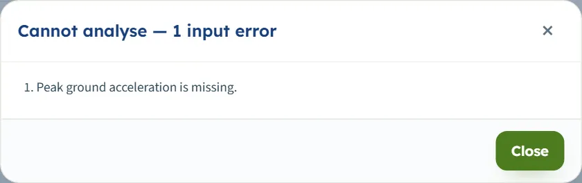
Before it calculates, the module checks the inputs. If one cannot be used, a window Cannot analyse — n input error(s) lists the messages, nothing is calculated, and the bar stays Not analysed. Fix the values and press Analyze again.
| When | Message |
|---|---|
| amax is zero | “Peak ground acceleration is missing.” |
| Mw is zero | “Moment magnitude is missing.” |
| ER is zero | “Hammer energy ratio is missing.” |
| FSreq is zero | “Required factor of safety is missing.” |
| A test lies below the profile | “BH-1 test 13 at 25 m lies below the profile (20 m).” |
| A unit weight is zero | “BH-1 layer 2: unit weight is missing.” / “… saturated unit weight is missing.” |
Several problems appear together in one window. A box left empty is not an error: it returns to its last value. The warnings that do not stop the run are in the Results section above.
Messages of the files and the template
- Import: “Edit inputs first — the import replaces the boreholes.” while results are shown.
- Import window problems: “BH-1: groundwater depth is missing.”, “BH-1!E8: unit weight γ is missing.”, “BH-1!K8: SPT N30 is missing.” (the row is skipped), “Sections!B7: "BH-9" is not a borehole of this file.”, “BH-1: the header row "From (m) · To (m) · USCS …" was not found — the sheet is skipped.” and, without a Project sheet, “No "Project" sheet — the earthquake, corrections and settings of the model are kept.” Replace the boreholes is offered unless an input error remains.
- A file that is not a workbook: “Not a GeoTerva template: not a zip (.xlsx) file”.
- Open file: “Not a model file: no boreholes found in the file”.
- “The project keeps at least one borehole.”
Good practice and common mistakes
- Give the groundwater depth of each borehole. Tests above it are not evaluated; the depth sets σ′v and so both CSR and CRR.
- Enter the raw N30 . The module applies the corrections; correcting twice lowers the answer.
- Give ER from the hammer record (60 % when unknown is the example default), and the real borehole diameter and sampler.
- Check the screening. Layers of PI at or above the limit are not evaluated: look at the Warnings and check them for cyclic softening separately.
- Use laboratory fines (FC lab) for tests that have them; the layer value is the fallback.
- Make one section per line and give the true distances; use Columns to look at the boreholes alone.
- Check amax and Mw — they are your inputs and the answer is sensitive to them (table above).
- Save to a file for the project record: the browser store is only in this browser.
Frequently asked questions
How is the factor of safety against liquefaction calculated here?
FS = CRR / CSR at every test below the groundwater table, with CSR = 0.65 · (σv/σ′v) · amax · rd and CRR from the clean-sand equivalent corrected blow count, scaled for magnitude and overburden. For BH-1 at 4.00 m: CSR 0.3087, CRR 0.1413, FS 0.46.
When is a test triggered, marginal or OK?
Below 1.0 it is triggered; from 1.0 up to the required factor of safety (1.20 by default) it is marginal; at or above it, OK.
Why are some tests “not evaluated”?
They lie above the groundwater table, deeper than the deepest test (20 m by default) or in clay-like soil (PI at or above the limit, 7 by default; CL, CH, OL, OH, PT when PI is blank). They stay in every table with the reason.
Which method does it use?
Idriss & Boulanger (2014) for SPT: corrected blow count with energy, diameter, sampler and rod-length factors, overburden and fines corrections, and the magnitude and overburden scaling of the same reference.
Can I analyse several boreholes at once?
Yes. Any number of boreholes in one project; the results table, the project summary and the sections show them together.
How do I draw a section between boreholes?
In Sections press Add section, add the boreholes and give each its distance along the line. The Contours view then draws colour bands between them; without a section it draws one colour column per borehole.
Does the module keep my project?
Yes. Every change is kept in the browser and the page opens with the project you last worked on, analysed or not. Save to file, Quick Save and Reset to defaults are in Model data.
How do I use the Excel template?
Download it (filled with your model), edit the Project, Sections and borehole sheets, and import it. A window lists what was found and the problems before anything is replaced.
Which units can I use?
SI · kN, SI · tf or US, switchable in the header even after Analyze. The drawings stay in SI; the cards, tables, boxes and calculations convert. The Excel template is always metres, kN/m³, % and g.
Where do I enter the magnitude and the acceleration?
In Earthquake: the peak ground acceleration in g and the moment magnitude. They are your inputs for the whole project.
What does the report contain?
A cover, then introduction and scope, boreholes and soil profiles, earthquake and settings, results by borehole with figures, test by test tables, warnings when there are any, and a summary. Save it as PDF or download it as Word after Analyze.
Does it check settlement or lateral spreading?
No: the module gives triggering. Settlement, lateral spreading and loss of bearing capacity are separate checks that use the zones it finds.