

What the module calculates
CPT triggering checks whether liquefaction is triggered at every reading of a cone penetration test below the groundwater table. You enter one or several CPT soundings (or fill in the Excel template), the design earthquake (a peak ground acceleration and a moment magnitude) and a method. For each reading the module finds the cyclic stress ratio CSR (what the earthquake asks of the soil), the cyclic resistance ratio CRR (what the soil can give), and the factor of safety:
FS below 1.0 is a triggered reading; FS from 1.0 up to the required value FSreq is marginal; at or above FSreq it is OK. Readings the procedure does not apply to (above the design water table, clay-like, deeper than a limit you set) are listed as not evaluated.
What you can describe
- Several soundings in one project, each with its own groundwater depth, ground elevation and readings (depth, cone resistance qc, sleeve friction fs, and the pore pressure u2 when recorded).
- Two methods, each a complete package: Boulanger & Idriss (2014) and Robertson & Wride (1998).
- Sections: lines through some of the soundings, with the distance of each along the line, for the colour-band drawings.
- Excel in and out: a template with a Project sheet, a Sections sheet and one sheet per sounding.
The module gives, for every sounding, the soil behaviour log, the profile of qc1Ncs , CSR, CRR and FS against depth, the triggered and marginal zones with their thickness, colour-band sections between the soundings, a project summary, a step-by-step calculation of any reading, and a PDF or Word report.
Which module for which job
- This module starts from cone data. The soil type, the unit weight and the fines content are estimated from qc, fs and u2, so no samples are needed to run it.
- For SPT blow counts, boreholes with fines content and unit weights, use the SPT triggering manual.
Before you start: what you need
Have these ready:
| What | Notes |
|---|---|
| The CPT readings | Depth, cone resistance qc and sleeve friction fs for every reading. The pore pressure u2 behind the cone is used when you have it. If the file holds the corrected cone resistance qt or a friction ratio instead, the import and the paste dialog convert them. |
| The groundwater depth of each sounding | The depth at the time of the test. A different design depth can be entered for each sounding. |
| The ground elevation of each sounding | Needed for the sections: the soundings are placed at their elevations. |
| The design earthquake | The peak ground acceleration amax at the ground surface, in g, and the moment magnitude Mw. Both are your inputs. |
| Where the soundings lie | For a colour-band section: the distance of each sounding along a line. |
Quick start in eight steps
- Open the module and choose the units
Open CPT triggering from the Liquefaction family. Pick SI · kN, SI · tf or US in the header; you can change it at any time.
- Bring the soundings in
Either download the template from Excel input, fill one sheet per sounding and press Import Excel…, or choose a sounding under Soundings and use Paste readings… in Cone readings.
- Set the groundwater and the sections
For each sounding enter the groundwater depth (and the elevation). In Sections give each sounding its distance along a section.
- Enter the earthquake
In Earthquake type amax and Mw.
- Choose the method
In Analysis Settings pick Boulanger & Idriss (2014) or Robertson & Wride (1998) and review the unit weight, FSreq and the screening limits.
- Press Analyze
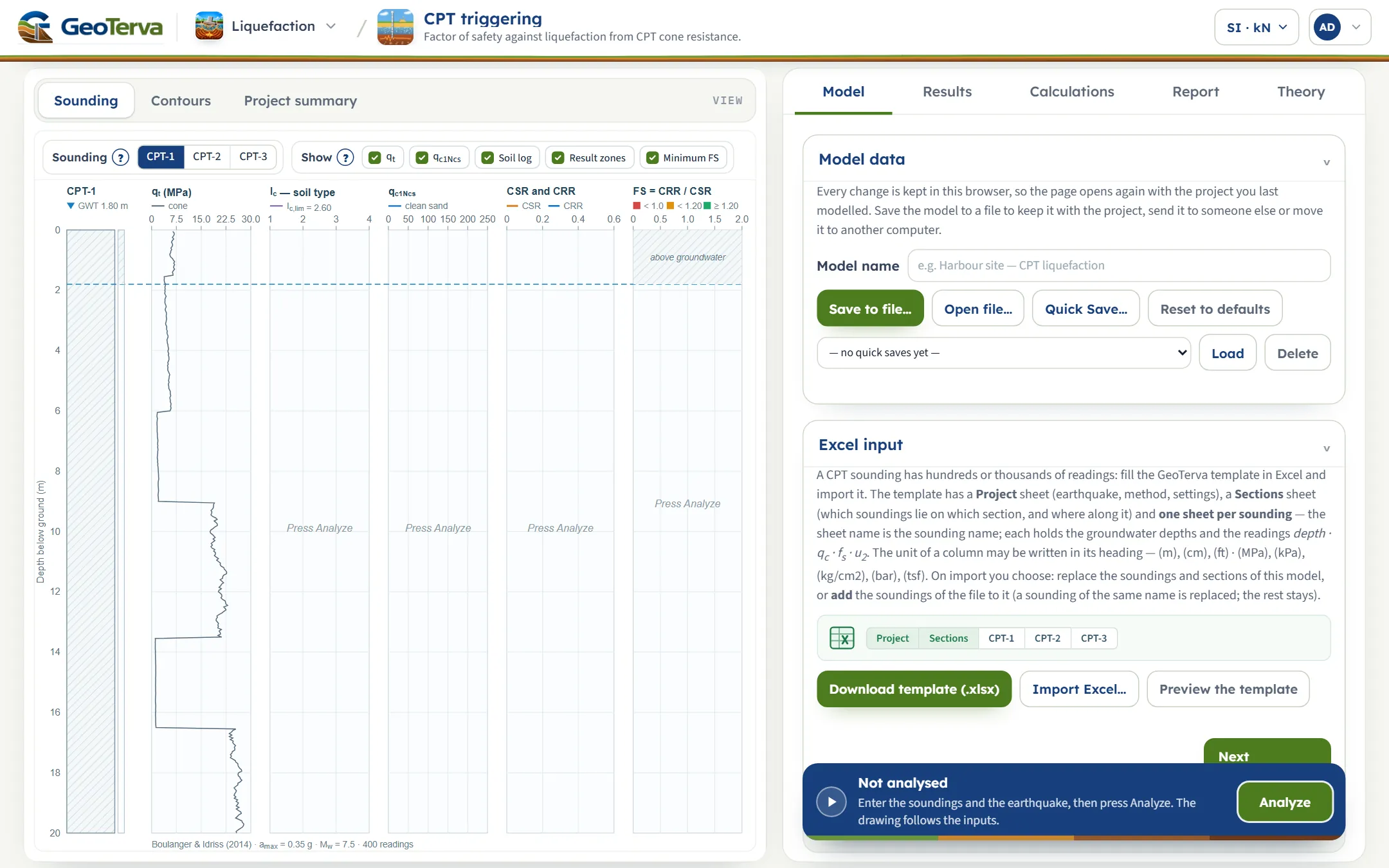
Press Analyze at the foot of the Model tab. The inputs lock, the drawing changes to Contours, and a Warnings window opens if the run has warnings.
- Read the answer
The Results tab gives the result of each sounding and a table reading by reading; the Sounding and Project summary views show the same against depth. Click a depth to open its calculation.
- Take the report
The Report tab saves a PDF or a Word file.
The screen: three views of the project
The layout is the one every GeoTerva module shares, described in the workspace guide: drawings on the left, the Model, Results, Calculations, Report and Theory tabs on the right, and the Analyze bar at the foot of the Model tab. This module has three views, chosen with the buttons above the drawing.
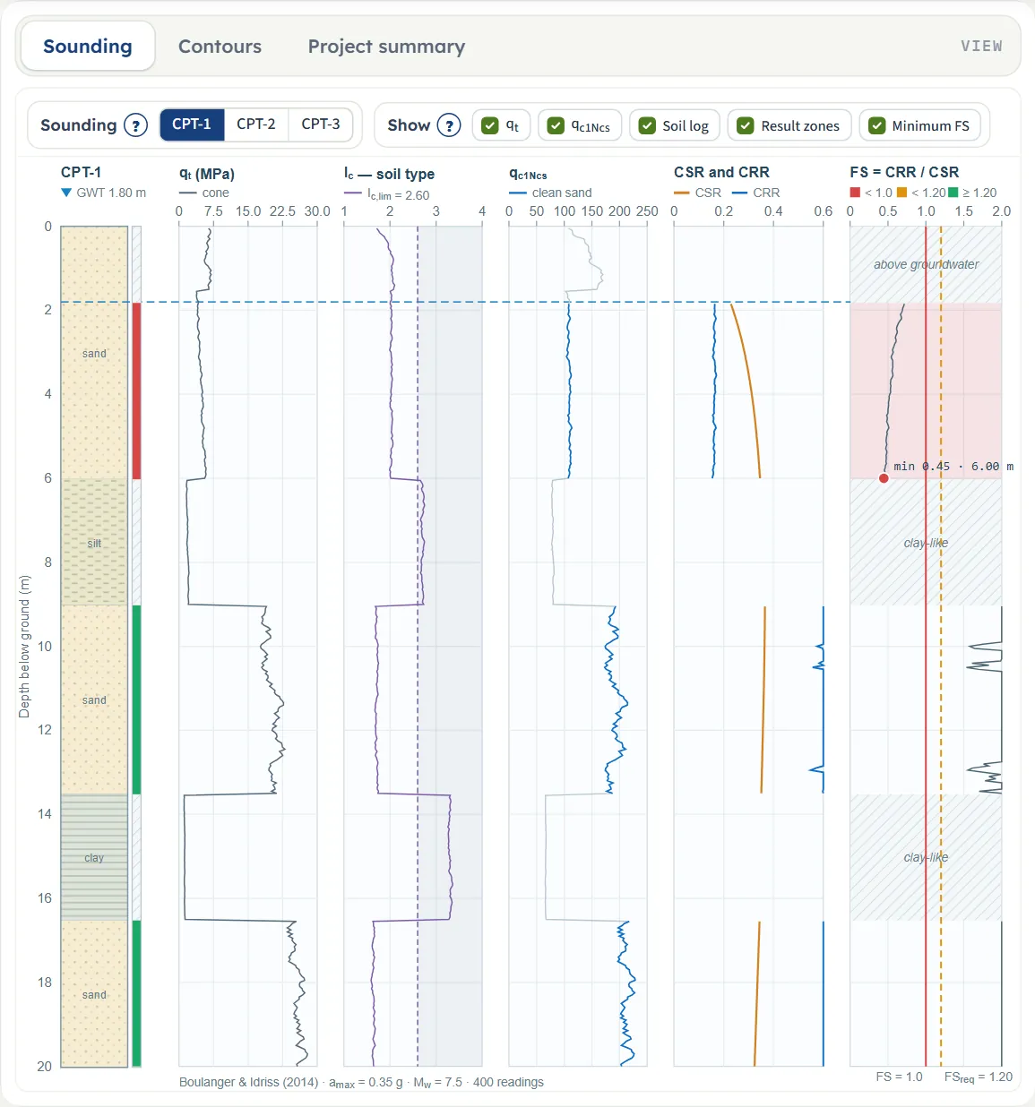
Sounding
One sounding at a time, chosen with the buttons beside Sounding. From the left: the soil behaviour log with the result strip beside it, then five panels against depth: the cone resistance qt, the soil behaviour index Ic with the clay-like limit, the clean-sand cone resistance qc1Ncs , CSR and CRR, and FS with the lines at FS = 1.0 and at FSreq . The groundwater depth is the dashed blue line; ranges that are not evaluated are hatched and named (above groundwater, clay-like), and the lowest FS is marked with its value and depth.
The Show chips switch qt, qc1Ncs , Soil log, Result zones and Minimum FS. They change the drawing only; the analysis always uses every reading. Before Analyze the cone resistance is drawn and the other panels say “Press Analyze”. Click any depth in the panels after Analyze and the Calculations tab opens at the nearest reading.
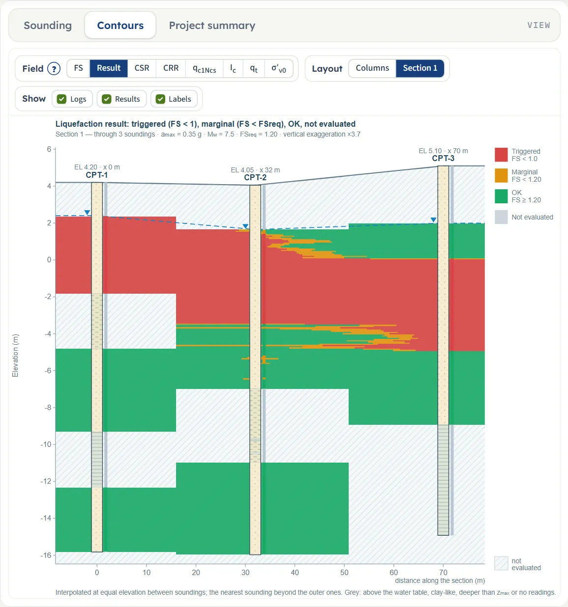
Contours
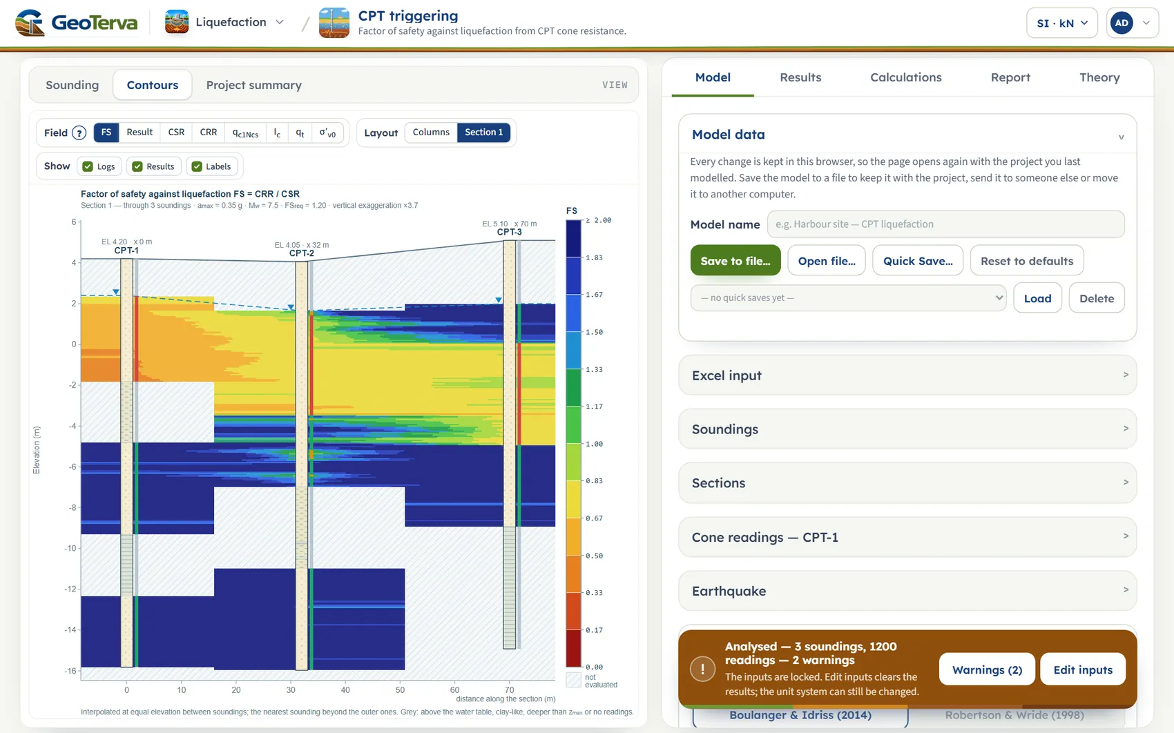
The colour-band section between the soundings of the chosen section. Each sounding gives the field against depth; between two soundings the field is interpolated linearly at equal elevation, and beyond the outer ones the nearest sounding is used. Grey is not evaluated. Three groups of chips sit above it:
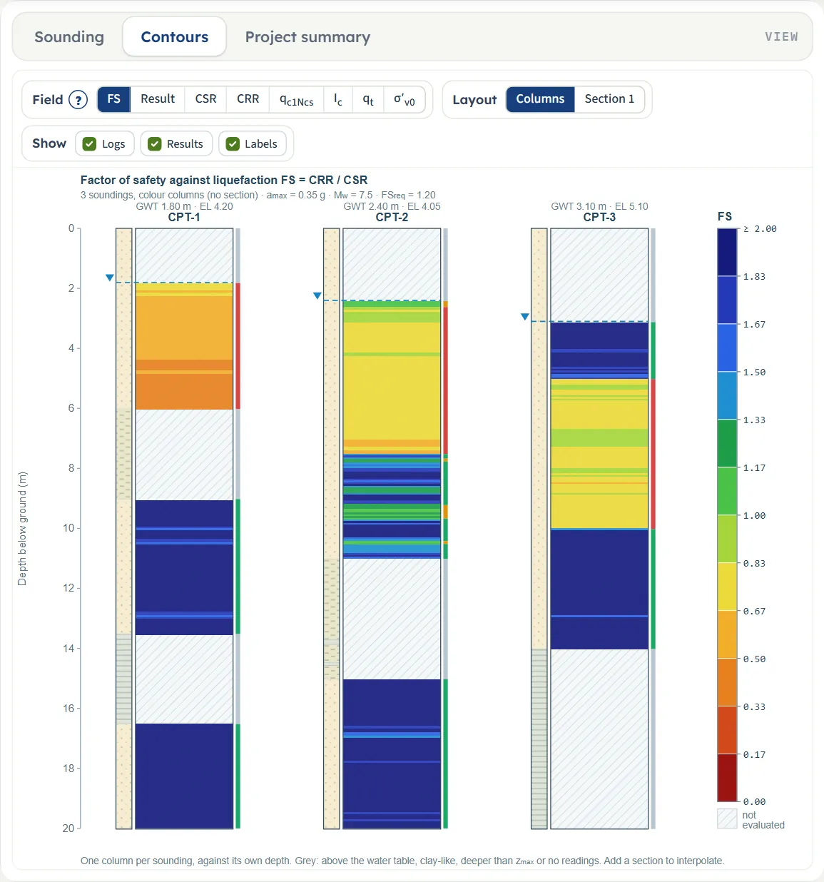
- Field: FS, Result (triggered, marginal, OK, not evaluated), CSR, CRR, qc1Ncs , Ic, qt and σ′v0 . FS runs on a fixed scale from 0 to 2 (2 and above at the top of the legend).
- Layout: Columns (one colour column per sounding against its own depth, no interpolation) or one chip per section; All appears when the project has two or three sections and draws them one under the other.
- Show: Logs (the soil log of each sounding), Results (the result strip) and Labels (name, elevation and distance).

Project summary
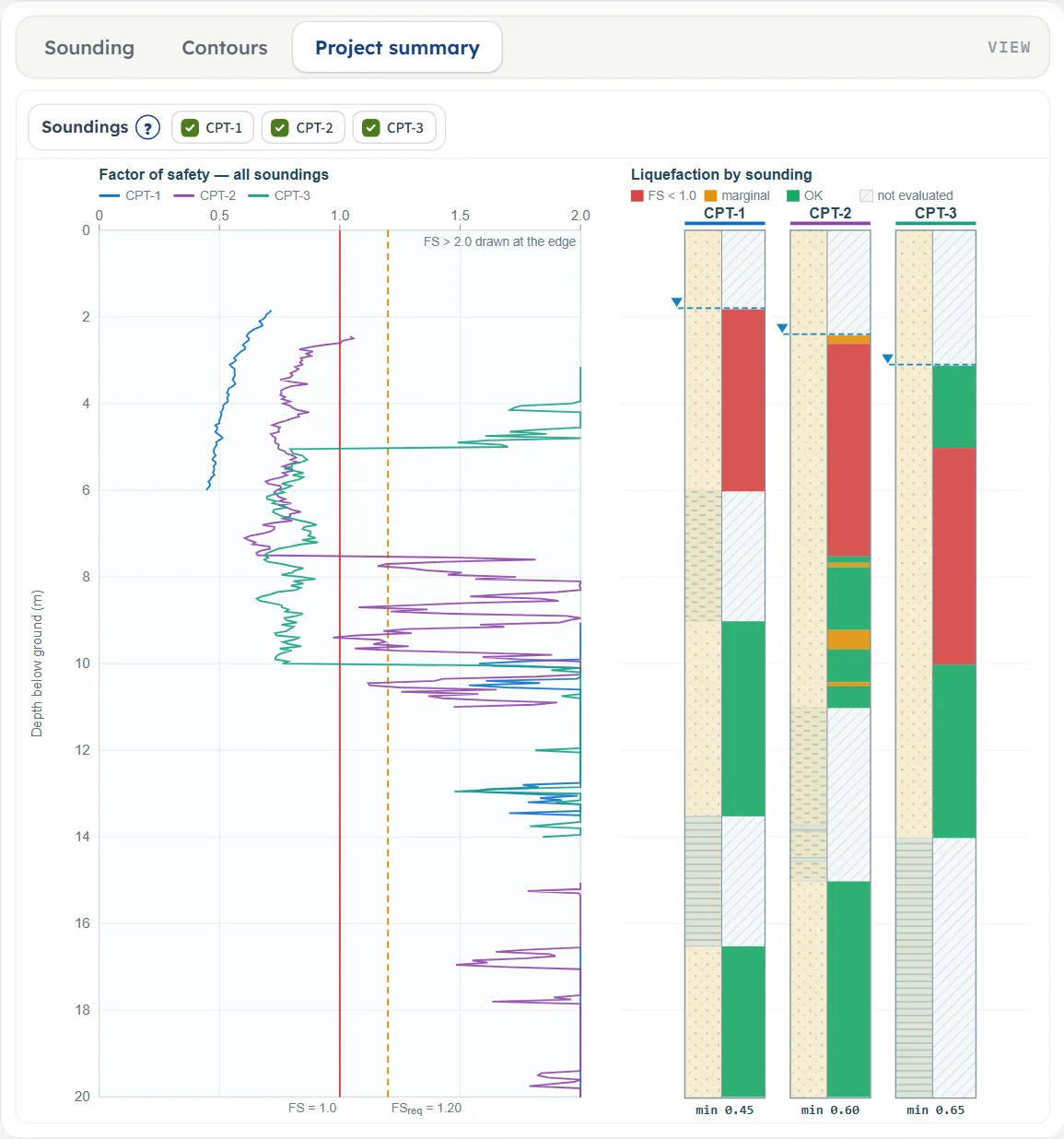
The factor of safety of every sounding on one plot, with the lines at 1.0 and FSreq (values above 2.0 are drawn at the edge), and on the right one column per sounding with its soil log and its result strip, the groundwater mark and the minimum FS written under it. The chips switch each sounding on or off.
Entering the model, section by section
The Model tab walks you through its sections: Model data stands on its own, and the others open one at a time with Back and Next at their foot: Excel input, Soundings, Sections, Cone readings, Earthquake and Analysis Settings. Opening one closes the previous one. After Analyze the inputs are locked until you press Edit inputs; the unit system can still be changed.
Model data
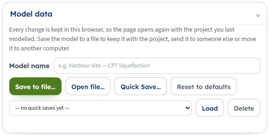
The box where the work is kept. Every change is kept in this browser: after a reload the module opens on the project you last worked on, analysed or not, and says so (“Opened with the project you last worked on …”). Model name is a label that goes into file names.
- Save to file… writes the model as a .gtrv file (in SI, whatever the page shows; the report cover is included). Where the browser offers it you choose the folder; otherwise the file goes to the download folder.
- Open file… reads such a file back and reports what it ignored.
- Quick Save… asks for a name and keeps this version in the list under it; choose it and press Load, or Delete it (after a confirmation). A name already used asks whether to replace it.
- Reset to defaults goes back to the example project: “The inputs are back at the module defaults, and this is now the model kept in the browser.”
Excel input
A CPT sounding has hundreds or thousands of readings, so the module works with a template. Download template (.xlsx) gives a workbook filled with the current model; Preview the template shows its first rows on the screen. The strip of tabs shows the sheets: Project, Sections and one sheet for each sounding.
- Project: amax , Mw, the method, CFC , f, a, the unit weight option and values, FSreq , Ic,lim , zmax and hmin .
- Sections: one row for every sounding of a section: the section name, the sounding and its distance along the line (m).
- One sheet per sounding: the sheet name is the sounding name; on top the groundwater depth during the test, the design groundwater depth (blank: the same) and the ground elevation; below the heading row the readings depth · qc · fs · u2.
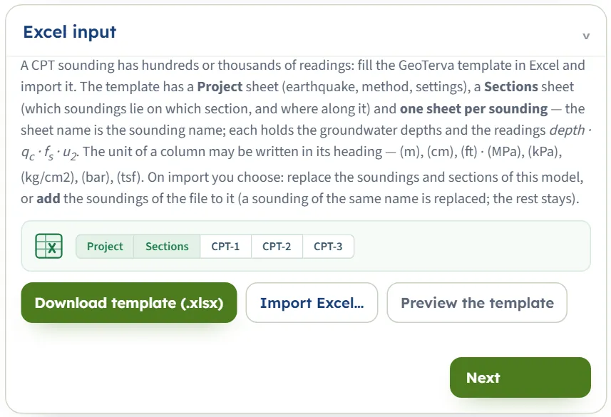
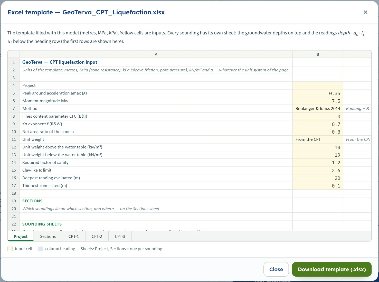
The template is always written in metres, MPa (cone resistance), kPa (sleeve friction and pore pressure), kN/m³ and g. On import the unit of a column may be written in its heading, in brackets: (m), (cm), (mm), (ft) for the depth and (MPa), (kPa), (kg/cm2), (bar), (tsf), (psi), (atm) and others for the stresses. A corrected cone resistance column qt is turned back into qc with the net area ratio, and a friction ratio column Rf into fs.
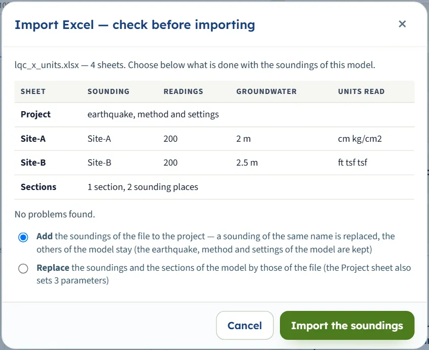
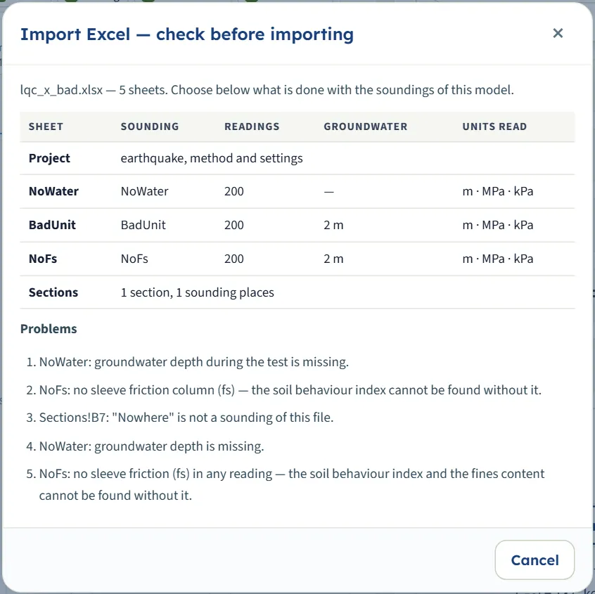
Press Import Excel… and choose the file. The module does not import at once: a window Import Excel — check before importing lists each sheet with its sounding, the number of readings, the groundwater depth and the units it read, and then either “No problems found.” or a numbered list of Problems. Without problems you choose:
- Add the soundings of the file to the project: a sounding of the same name is replaced, the others stay, and the earthquake, method and settings of the model are kept. The module then says, for example, “Added 2 soundings from …; the project has 5 soundings now.”
- Replace the soundings and the sections of the model by those of the file; the Project sheet then also sets its parameters (“Imported 2 soundings and 1 section from …”).
With problems the window offers only Cancel and the message under the buttons reads “The file could not be imported — see the problems.” A problem is, for example, a sounding sheet with no groundwater depth, no sleeve friction column, or a section row naming a sounding that is not in the file. Import is not possible while the model is analysed: press Edit inputs first.
Soundings
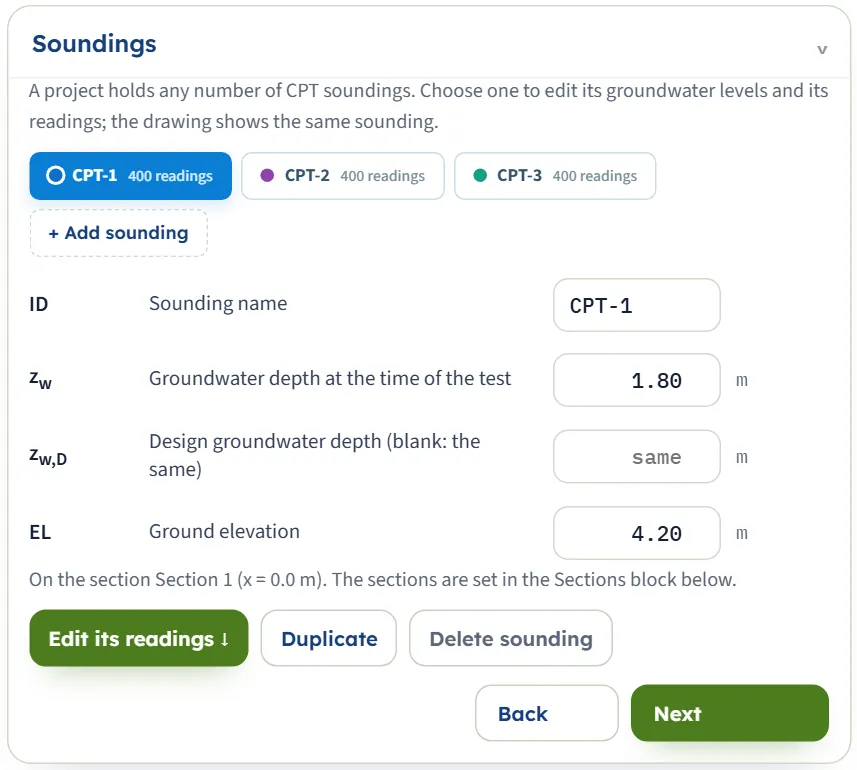
A project holds any number of soundings. The buttons list them with their number of readings (and, after Analyze, their result); the one you choose is the one in the drawing and in the readings table. + Add sounding adds an empty one: its groundwater depth is blank and it has no readings (its elevation is copied from the sounding you were on), so the analysis asks for both. Duplicate copies the chosen sounding; Delete sounding removes it (the project keeps at least one).
| Field | Notes |
|---|---|
| Sounding name (ID) | First sounding: CPT-1. Up to 24 characters. A name already used by another sounding is not accepted: the box goes back to the old name and a message says the name is already used. The name is also the sheet name in Excel. |
| Groundwater depth at the time of the test zw m · ft | First sounding: 1.80 (CPT-2 2.40, CPT-3 3.10). Used for the pore pressure at the time of the test, that is for the normalisation of the cone resistance. The box accepts 0 or more; a blank is not accepted. |
| Design groundwater depth zw,D m · ft | First sounding: blank (“same”). Used for CSR and Kσ. Blank means the same as zw. Also the depth above which readings are not evaluated. |
| Ground elevation EL m · ft | First sounding: 4.20 (CPT-2 4.05, CPT-3 5.10). Places the soundings in the Contours view. |
The default values of the three example soundings are listed in the table; a sounding you add has no groundwater depth until you enter one.
Sections
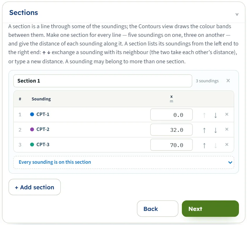
A section is a line through some of the soundings, and the Contours view draws one section at a time (or all, when there are two or three). + Add section makes a new, empty one, named “Section 2” and so on. In each section card: its name (editable), the list of its soundings from the left end to the right with the distance x of each along the line, ↑ ↓ to exchange a sounding with its neighbour (the two take each other’s distance), × to take a sounding out of the section, and a list at the foot to add a sounding that is not yet in it. A sounding may belong to more than one section. Typing a new distance puts the sounding in its place along the line. The default section is “Section 1”: CPT-1 at 0 m, CPT-2 at 32 m, CPT-3 at 70 m.
Cone readings
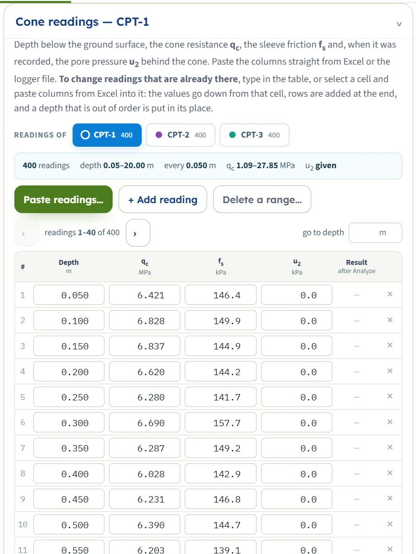
The readings of the sounding you chose (the buttons under Readings of change it). A summary line gives the number of readings, the depth range, the usual interval, the range of qc, whether u2 is given, and the number of gaps in the record. The table is paged (40 rows); go to depth jumps to a depth. Once analysed, each row shows its result, and clicking it opens its calculation.
- Type in the table. Enter and the arrow keys go along a column, Tab goes along the row. A depth typed out of order is put in its place.
- Paste into the table. Select a cell and paste columns from Excel: the values go down and to the right from that cell, rows are added at the end, and a heading row is skipped. The values are read in the units the table shows.
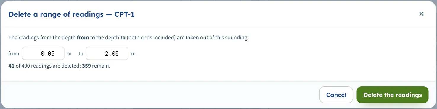
- Paste readings… opens the paste window (below). + Add reading adds a copy of the last reading one step deeper, to be edited. Delete a range… takes out the readings between two depths.
- The × on a row deletes it (not below three readings).
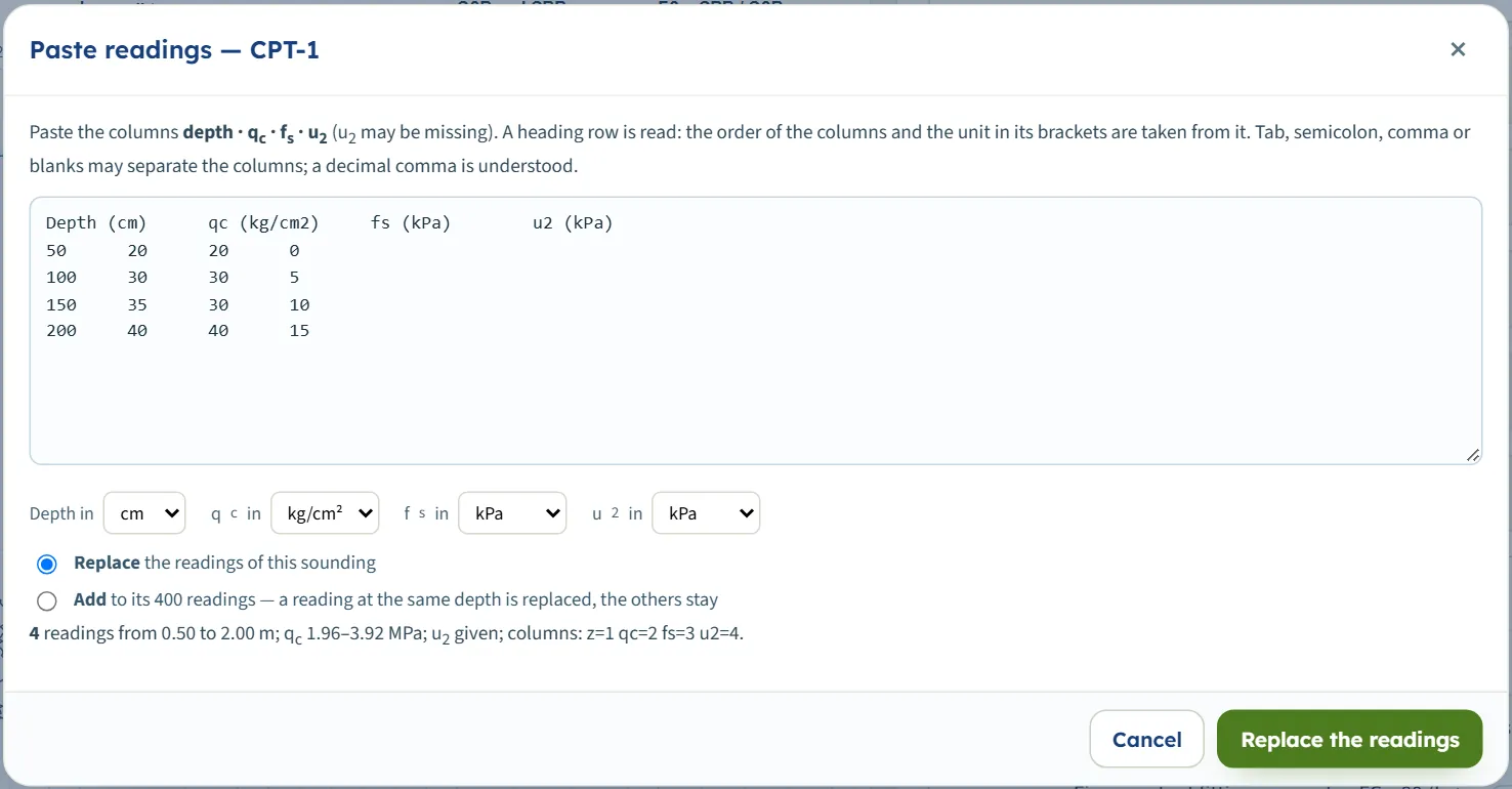
The paste window
Paste readings reads the text you paste: columns depth · qc · fs · u2 (u2 may be missing), separated by tabs, semicolons, commas or blanks, with a decimal point or comma. A heading row sets the order of the columns and the unit in its brackets; the four unit boxes below show what was understood, and you can change them. A line under the boxes checks the paste (a unit in brackets that the module does not know, such as “(furlong)”, is named there with “check it”, and the box below is used): the number of readings, the depth and qc range, whether u2 is given and the columns found. Replace the readings of the sounding (at least three rows) or Add to them (a reading at the same depth is replaced, the others stay). A paste with no sleeve friction, or a qc above 150 MPa, or a depth beyond 150 m cannot be accepted: its button stays greyed, and the line says why.
Earthquake
The design earthquake of the whole project. Both values are yours; the module does not derive them.
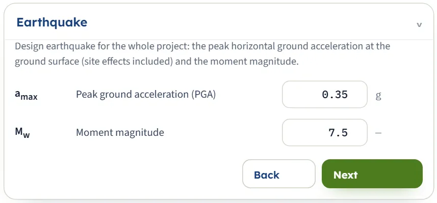
| Field | Default | Range |
|---|---|---|
| Peak ground acceleration (PGA) amax g | 0.35 | Above 0 and up to 2 g, at the ground surface, site effects included. |
| Moment magnitude Mw | 7.5 | 4 to 9.5. |
Analysis Settings
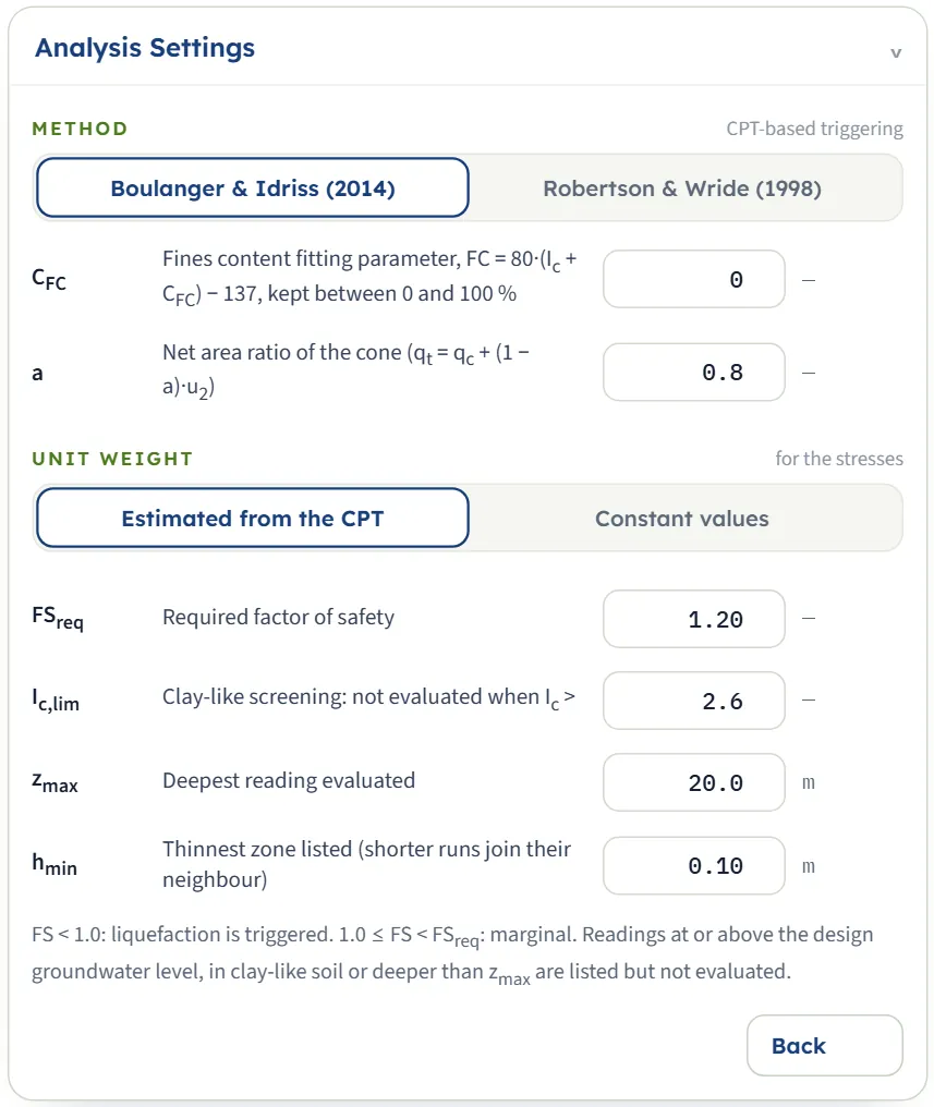
The method, the unit weight, and the limits of the screening. A box that does not apply is hidden: CFC shows only with Boulanger & Idriss, f only with Robertson & Wride, and the two unit weights only with Constant values.
| Field | Default | Range and effect |
|---|---|---|
| CFC | 0 | Fines content fitting parameter of Boulanger & Idriss: FC = 80·(Ic + CFC ) − 137, kept between 0 and 100 %. From −1 to 1; the correlation scatter is ±0.29. |
| f | 0.7 | Exponent of Kσ for Robertson & Wride, 0.5 to 1. |
| a | 0.8 | Net area ratio of the cone, above 0 up to 1: qt = qc + (1 − a)·u2. |
| γ, γsat kN/m³ · t/m³ · pcf | 18.0, 19.0 | Only with Constant values: above and below the groundwater level, 10 to 30 kN/m³. |
| FSreq | 1.20 | The limit between marginal and OK. Above 0, up to 5 (the box accepts from 0.01 to 5). |
| Ic,lim | 2.6 | Readings with Ic above it are clay-like and not evaluated. 1.5 to 3.6 (the box has the same limits). |
| zmax m · ft | 20.0 | The deepest reading evaluated. Above 0, at most 150 m (a larger value typed is taken as 150 m, one below 1 m as 1 m). |
| hmin m · ft | 0.10 | The thinnest zone listed: a run of one result thinner than this joins its longer neighbour. 0 to 5 m. |
Where a box needs a number and you clear it, the module keeps the previous value; a number outside the range the procedures were built for is not clipped silently but stops the analysis with a message (see Messages). The unit weights are only accepted in kN/m³ terms (10 to 30): a value of 1.9 typed in t/m³ in the SI · kN system is refused.
Choosing the method and the options
The two methods are two complete packages: each has its own stress reduction factor rd, its normalisation of the cone resistance, its clean-sand adjustment, its magnitude scaling factor and its Kσ. Do not mix their steps; choose one and read the result with it.
- Normalisation. Boulanger & Idriss: CN = (Pa/σ′v) raised to an exponent m that is found from qc1Ncs by iteration, at most 1.7. Robertson & Wride: CQ = (Pa/σ′v) raised to the exponent n of Ic, at most 1.7.
- Clean-sand value. Boulanger & Idriss: qc1Ncs = qc1N + Δqc1N , with the fines content FC from Ic and CFC . Robertson & Wride: (qc1N)cs = Kc · qc1N , with Kc from Ic.
- Stress reduction rd. Boulanger & Idriss: depends on depth and Mw. Robertson & Wride: depends on depth only.
- Magnitude scaling MSF. Boulanger & Idriss: depends on qc1Ncs and Mw. Robertson & Wride: 102.24 / Mw2.56 .
- Overburden factor Kσ. Boulanger & Idriss: from qc1Ncs and σ′v, at most 1.1. Robertson & Wride: (σ′v/Pa)f−1 above one atmosphere, otherwise 1.
With the default example the two methods give, at the same reading, FS = 0.52 (Boulanger & Idriss) and 0.49 (Robertson & Wride); see the worked example. Over the whole example the lowest factor of safety of CPT-1, CPT-2 and CPT-3 is 0.45, 0.60, 0.65 with Boulanger & Idriss and 0.42, 0.64, 0.68 with Robertson & Wride.
Unit weight
- Estimated from the CPT (the default): the unit weight of every reading is found from Rf and qt (kept between 1.5 and 2.5 times the unit weight of water) and integrated down to the stresses. No sample data needed.
- Constant values: γ above and γsat below the groundwater level. Use it when you have measured unit weights you trust more. With 18 and 19 kN/m³ the example changes little: the lowest FS is 0.45, 0.61, 0.66.
The screening limits
- Ic,lim decides what counts as clay-like. The default 2.6 leaves out the silt mixtures and clays of the example. Raising it to 3.0 brings readings of silty soil into the evaluation, and the lowest FS of CPT-1 and CPT-2 falls to 0.32 (triggered thickness of CPT-1: 7.20 m instead of 4.20 m). Where evaluated readings have Ic between 2.4 and the limit, a warning lists them.
- zmax limits the depth of the evaluation.
- FSreq moves the border between marginal and OK; it changes no FS.
- hmin only tidies the zones: thin runs join their neighbours in the zones and in the thicknesses, not in the readings.
Analyze and read the results
Press Analyze. The bar counts through the soundings (“Analysing… CPT-1 (1 / 3)”) and then reads Analysed — 3 soundings, 1200 readings, with the number of warnings when there are some, and “The inputs are locked. Edit inputs clears the results; the unit system can still be changed.” The module stays on the Model tab; the drawing changes to Contours, a short message says “Analysed — the colour bands show the selected field; see also the Sounding view and the Results tab.”, and when the run has warnings the Warnings window opens by itself. Open the Results tab for the answer.
The Results tab
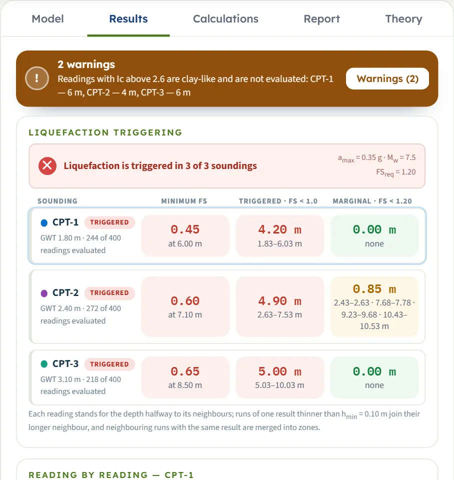
At the top a banner gives the verdict of the project in words: “Liquefaction is triggered in 3 of 3 soundings”, “Not triggered, but marginal (FS below 1.20) in 1 of 3 soundings”, “Liquefaction is not triggered in any sounding”, or “No reading could be evaluated — no factor of safety”, with amax , Mw and FSreq . Under it, one row for each sounding (click it to show the sounding in the drawing and in the table below):
| Cell | What it is |
|---|---|
| Name and chip | The sounding, its groundwater depth and how many readings were evaluated. The chip is TRIGGERED (any reading with FS below 1.0), MARGINAL (none triggered, some below FSreq ) or OK. |
| Minimum FS | The lowest FS of the sounding and its depth. |
| Triggered · FS < 1.0 | The total thickness of the triggered zones and the zones themselves (the first four, then “+ n more”). |
| Marginal · FS < 1.20 | The same for the marginal zones (the limit is your FSreq ). |
Each reading stands for the depth halfway to its neighbours (at most a quarter of a metre either side, or three quarters of the usual interval where that is larger), so a gap in the record is not filled with results. Neighbouring runs with the same result are merged into zones.
Reading by reading
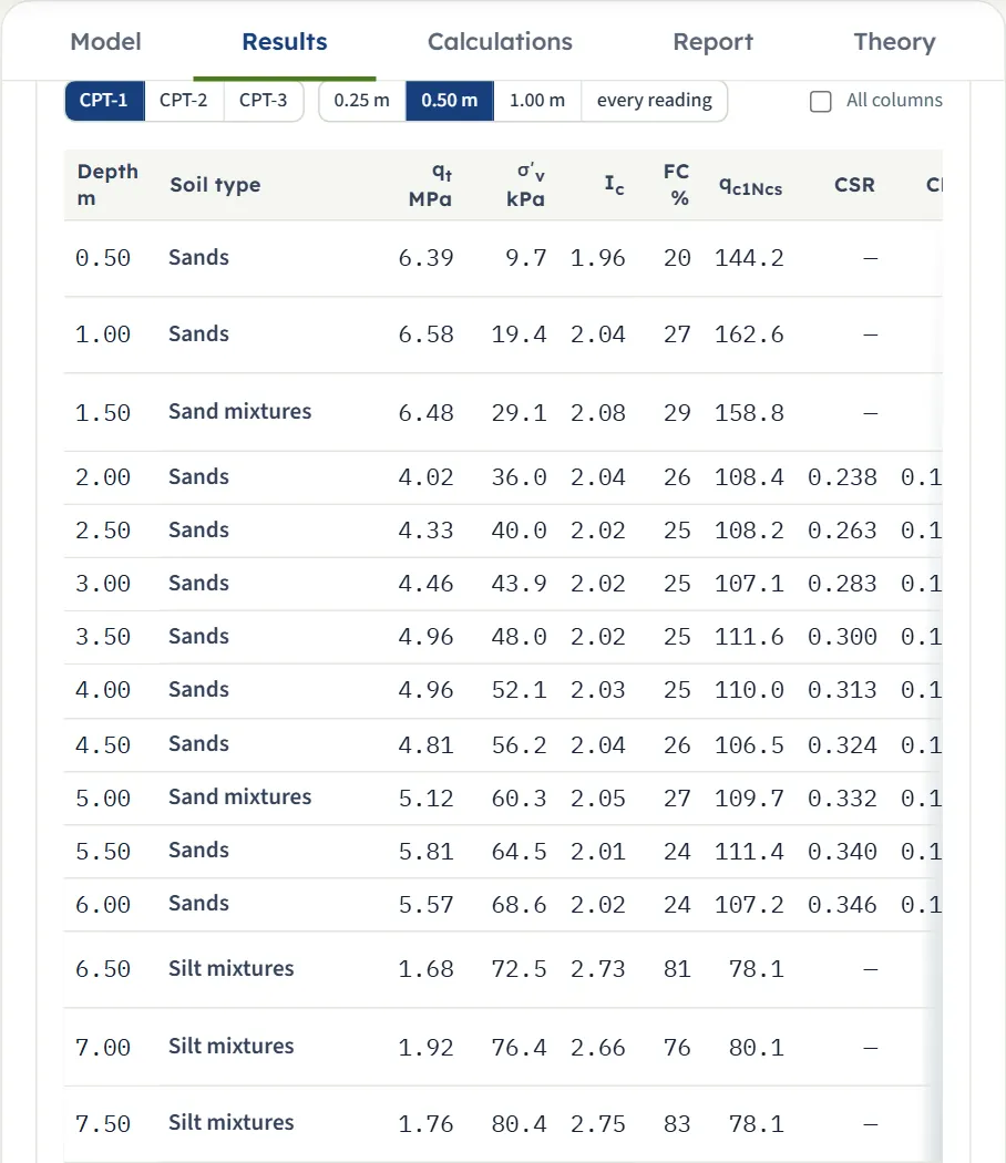
Below the rows, the readings of the chosen sounding in a table. The buttons choose the sounding and the depth step (0.25 m, 0.50 m, 1.00 m or every reading; the labels follow the unit system). The default columns are the depth, the soil type, qt, σ′v, Ic, FC, qc1Ncs , CSR, CRR, FS and the result; All columns adds fs, Rf, γ, σv, n, the normalisation factor, qc1N , the clean-sand adjustment, rd, CRR7.5 , MSF and Kσ. A reading that is not evaluated shows N/E and the reason under the chip. Click a row to open its calculation.
The Warnings window
Warnings (n) (on the Analyze bar and on the warning banner) opens a window with the numbered warnings of the run and, below them, the assumptions of this analysis: the method and its formulas, how the unit weight was found, which groundwater depth each step uses, the screening and the zone rule. The default example has two warnings:
- “Readings with Ic above 2.6 are clay-like and are not evaluated: CPT-1 — 6 m, CPT-2 — 4 m, CPT-3 — 6 m. Check these layers for cyclic softening separately.”
- “q₁Ncs ≥ 211, taken at the upper limit of the CRR curve (thickness of the readings concerned): CPT-1 — 1.9 m; CPT-2 — 0.05 m.”
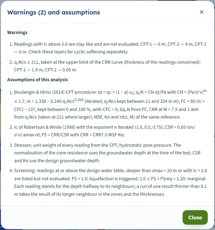
A warning does not stop anything: the numbers are there. Read it as a note on what the result rests on. Press Edit inputs to unlock the model and clear the results; the view returns to Sounding.
The Calculations tab, the report and the Theory tab
Calculations
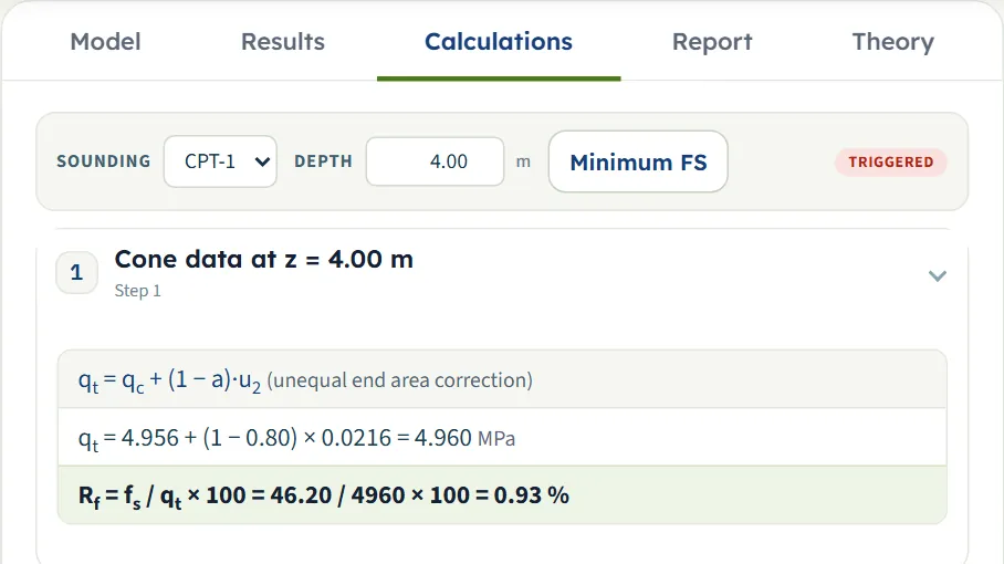
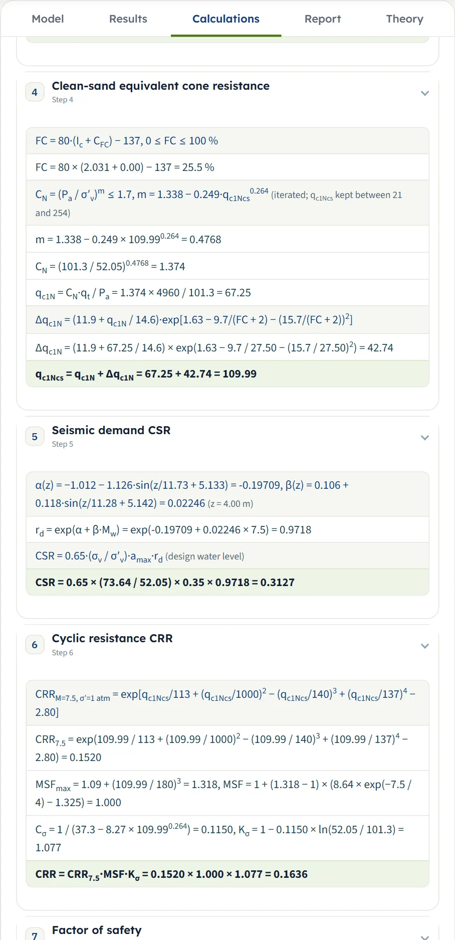
The Calculations tab writes out the working for one reading with your numbers. Choose the sounding and the depth at the top (the nearest reading is used), press Minimum FS to jump to the lowest FS of the sounding, or arrive by clicking a depth in the Sounding view or a row of a table. The tab opens on the minimum reading. Seven steps, each with its equation, the equation with your numbers, and the result:
- Cone data: qt = qc + (1 − a)·u2 and Rf.
- Vertical stresses: the unit weight, σv, the pore pressure u and σ′v0 , at the test and for the design water level.
- Soil behaviour type index Ic: the iteration on the exponent n and the soil type.
- Clean-sand equivalent cone resistance: FC, the exponent, the normalisation and the adjustment (or CQ and Kc for Robertson & Wride).
- Seismic demand CSR: rd and CSR.
- Cyclic resistance CRR: CRR7.5 , MSF and Kσ (with the limits applied shown in the line).
- Factor of safety: FS = CRR / CSR and the word (triggered, marginal, OK). A reading that is not evaluated stops after the normalisation and says why.
Before Analyze the tab says “Press Analyze on the Model tab first.” Each step folds and unfolds with its heading.
The report
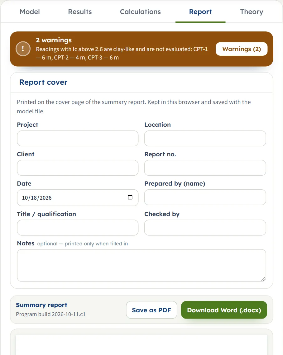
In the Report tab fill in the cover: project, location, client, report number, date (today’s date at the start), prepared by, title or qualification, checked by, and optional notes. The details are kept in the browser and saved with the model file. After Analyze, Save as PDF (it opens a print window; allow pop-ups and choose “Save as PDF” as the printer) and Download Word (.docx) are available; before it they are greyed out and the preview says “Open this tab after the analysis to build the preview.” or asks you to press Analyze. The preview is the report itself.
The report has a cover with the key results and a one-sentence conclusion, then the parts 1 Introduction and scope, 2 Soundings (the table of soundings and the table of sections), 3 Earthquake, method and settings, 4 Results by sounding (the table of results with the colour-band drawing of each section and the project drawing), 5 Reading by reading (for each sounding a table of readings every 0.50 m and its drawing), 6 Warnings (only when the run has warnings) and Summary. It states the units of the unit system you had chosen.
The Theory tab
The Theory tab has sixteen sections: the scope, the cone data, unit weight and stresses, the soil behaviour index, the screening, the two methods, the cyclic stress ratio, the factor of safety, the zones, the colour-band section, a comparison of the two methods, a worked reading computed from the example, the limits of the module and the references. The first three are open; the others open with their headings or from the contents list.
Worked example: the module’s own example
The module opens on this project: three soundings of 400 readings each (every 0.05 m to 20 m), amax = 0.35 g, Mw = 7.5, Boulanger & Idriss, the unit weight from the CPT, FSreq = 1.20. The results are those in the Results tab: CPT-1 minimum FS 0.45 at 6.00 m; CPT-2 minimum FS 0.60 at 7.10 m; CPT-3 minimum FS 0.65 at 8.50 m (all three triggered; triggered thickness 4.20, 4.90 and 5.00 m).
One reading by hand: CPT-1 at 4.00 m
Open the Calculations tab on CPT-1 at 4.00 m: qc = 4.956 MPa, fs = 46.2 kPa, u2 = 21.6 kPa, groundwater at 1.80 m. The numbers below are the module’s, and each was re-computed by hand.
| Step | Working | Result |
|---|---|---|
| qt, Rf | 4.956 + (1 − 0.8) × 21.6/1000; 46.2 / 4960 × 100 | 4.960 MPa; 0.93 % |
| Stresses | γ = (0.27 log 0.93 + 0.36 log(4960/101.3) + 1.236) × 9.81; u = 9.81 × (4.00 − 1.80) | γ = 18.01 kN/m³; σv = 73.64 kPa (the unit weights integrated from the surface); u = 21.58; σ′v = 52.05 kPa |
| Ic | n = 1.0 gives 1.916 (below 2.6), so n = 0.5 is tried: 2.031, granular | Ic = 2.03, soil type Sands |
| FC | 80 × 2.031 − 137 | 25.5 % |
| Normalisation | m = 1.338 − 0.249 × 109.990.264 ; CN = (101.3/52.05)m; qc1N = CN × 4960/101.3 | m = 0.4768; CN = 1.374; qc1N = 67.25 |
| Clean sand | Δqc1N = (11.9 + 67.25/14.6) · exp[1.63 − 9.7/27.5 − (15.7/27.5)²] | Δqc1N = 42.74; qc1Ncs = 109.99 |
| CSR | rd = exp(α + β × 7.5) with α = −0.19709, β = 0.02246; 0.65 × (73.64/52.05) × 0.35 × 0.9718 | rd = 0.9718; CSR = 0.3127 |
| CRR | CRR7.5 = exp(109.99/113 + 0.10999² − (109.99/140)³ + (109.99/137)⁴ − 2.80); MSF = 1.000; Kσ = 1 − 0.1150 × ln(52.05/101.3) | CRR7.5 = 0.1520; Kσ = 1.077; CRR = 0.1636 |
| FS | 0.1636 / 0.3127 | 0.52: triggered |
The Results table gives FS = 0.52 for 4.00 m, and the lowest value of CPT-1, 0.45, is at 6.00 m (the Calculations tab opens there).
The same reading with Robertson & Wride
Choose Robertson & Wride (1998) and press Analyze again (after Edit inputs). At 4.00 m: Ic = 2.031 as before, CQ = (101.3/52.05)0.5 = 1.395, qc1N = 68.30, Kc = 1.343 (the quartic of Ic), (qc1N)cs = 91.73, CRR7.5 = 93 × 0.09173³ + 0.08 = 0.1518, rd = 1 − 0.00765 × 4.00 = 0.9694, MSF = 102.24 / 7.52.56 = 1.000, Kσ = 1.0 (the effective stress is below one atmosphere), CSR = 0.65 × (73.64/52.05) × 0.35 × 0.9694 = 0.3120, so FS = 0.1518 × 1.000 / 0.3120 = 0.49. The lowest FS of the three soundings is 0.42, 0.64, 0.68.
Checking the units
Switch to US after Analyze: the cards re-state without a new run. The groundwater depth of CPT-1 reads 5.91 ft, the lowest FS is the same 0.45 at 19.69 ft, the triggered thickness 13.78 ft (4.20 m) and hmin 0.33 ft. In the Calculations tab at 6.00 m (19.685 ft): qt = 58.210 tsf (5.574 MPa), σ′v0 = 1.434 ksf (68.64 kPa) and Pa = 2.116 ksf, and the factor of safety is again 0.45. In SI · tf the same step reads qt = 56.841 kg/cm² and σ′v0 = 6.999 t/m², the unit weight 1.84 t/m³, and again FS = 0.45. Only the units change; the drawings stay in SI.
How each input changes the answer
Each row changes one thing (two where the label says so) in the example: Boulanger & Idriss, amax = 0.35 g, Mw = 7.5, CFC = 0, a = 0.8, the unit weight from the CPT, FSreq = 1.20, Ic,lim = 2.6, groundwater as in the example (1.80, 2.40 and 3.10 m), and runs the module again. The numbers are the minimum FS of each sounding, as the Results tab gives them.
| Change | Lowest FS | Result |
|---|---|---|
| The example Boulanger & Idriss, 0.35 g, Mw 7.5 | 0.45 · 0.60 · 0.65 | triggered in 3 of 3 |
| amax = 0.15 g CPT-1 is marginal at the lowest point | 1.04 · 1.41 · 1.53 | marginal in 1 of 3 |
| amax = 0.25 g | 0.62 · 0.85 · 0.92 | triggered in 3 of 3 |
| amax = 0.45 g | 0.35 · 0.47 · 0.51 | triggered in 3 of 3 |
| Mw = 6.5 | 0.52 · 0.74 · 0.82 | triggered in 3 of 3 |
| Mw = 8.0 | 0.42 · 0.55 · 0.59 | triggered in 3 of 3 |
| Mw = 6.5 and 0.25 g | 0.72 · 1.04 · 1.15 | triggered in 1 of 3 |
| Robertson & Wride, f = 0.7 | 0.42 · 0.64 · 0.68 | triggered in 3 of 3 |
| Robertson & Wride, f = 0.9 Only CPT-3 changes at two decimals | 0.42 · 0.64 · 0.70 | triggered in 3 of 3 |
| 0.20 g, Boulanger & Idriss | 0.78 · 1.06 · 1.15 | triggered in 1 of 3 |
| 0.20 g, Robertson & Wride | 0.73 · 1.12 · 1.19 | triggered in 1 of 3 |
| CFC = +0.29 More fines in the correlation | 0.58 · 0.87 · 0.91 | triggered in 3 of 3 |
| CFC = −0.29 Fewer fines | 0.32 · 0.37 · 0.38 | triggered in 3 of 3 |
| CPT-1 water at 0.50 m (test and design) Only CPT-1 changes | 0.38 · 0.60 · 0.65 | triggered in 3 of 3 |
| CPT-1 water at 4.00 m (test and design) Only CPT-1 changes | 0.55 · 0.60 · 0.65 | triggered in 3 of 3 |
| CPT-1 design water at 0.50 m, test 1.80 m Only CPT-1 changes | 0.37 · 0.60 · 0.65 | triggered in 3 of 3 |
| γ = 18, γsat = 19 kN/m³ | 0.45 · 0.61 · 0.66 | triggered in 3 of 3 |
| a = 0.6 | 0.45 · 0.61 · 0.66 | triggered in 3 of 3 |
| Ic,lim = 3.0 Silty readings are evaluated | 0.32 · 0.32 · 0.65 | triggered in 3 of 3 |
Reading the table:
- The earthquake moves everything. Raising amax from 0.35 to 0.45 g lowers the lowest FS of CPT-1 from 0.45 to 0.35; at 0.15 g no sounding is triggered. A smaller magnitude raises FS through MSF: Mw 6.5 gives 0.52, 0.74, 0.82.
- The two methods agree to a few hundredths at the lowest points (0.42, 0.64, 0.68 against 0.45, 0.60, 0.65), and differ more in the zones: the marginal thickness of CPT-2 is 0.85 m with Boulanger & Idriss and 0.25 m with Robertson & Wride. At 0.20 g CPT-1 is triggered with both and CPT-2 and CPT-3 are marginal.
- CFC is a strong lever on silty sand. The ±0.29 range of the correlation scatter moves the lowest FS of CPT-2 from 0.37 to 0.87.
- A groundwater change moves only its own sounding, and both the level at the test and the design level matter: water at 0.50 m for CPT-1 gives 0.38, at 4.00 m 0.55.
- The unit weight option and the net area ratio shift the lowest FS by a hundredth or so in this example: 0.45, 0.61, 0.66 with constant weights, 0.45, 0.61, 0.66 with a = 0.6.
Some inputs change the zones and not the factor of safety:
| Change | Triggered | Marginal |
|---|---|---|
| The example | 4.90 | 0.85 |
| FSreq = 1.0 | 4.90 | 0.00 |
| FSreq = 1.5 | 5.00 | 1.75 |
| hmin = 0 | 4.95 | 0.75 |
| hmin = 0.5 m | 5.10 | 0.00 |
| zmax = 10 m | 4.90 | 0.75 |
The minimum FS of CPT-2 stays 0.60 in all of these rows.
Messages: when the module stops, and what it warns about
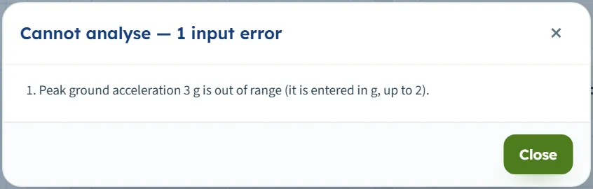
When a value cannot be used, Analyze stops: a window titled Cannot analyse — 1 input error (or “2 input errors”) lists the messages, nothing is calculated, and the Analyze bar stays on “Not analysed”. Correct the value and press Analyze again.
| Kind | When | Message |
|---|---|---|
| Stop | amax above 2 (or 0) | “Peak ground acceleration 3 g is out of range (it is entered in g, up to 2).” (0: “Peak ground acceleration is missing.”) |
| Stop | Mw outside 4 to 9.5 | “Moment magnitude 10 is out of range: the magnitude scaling factors are defined for 4 to 9.5.” |
| Stop | FSreq above 5 | “Required factor of safety 6 is out of range (up to 5).” |
| Stop | a outside 0 to 1 | “The net area ratio of the cone must be between 0 and 1.” |
| Stop | CFC beyond ±1 | “The fines content parameter CFC 2 is out of range (the correlation scatter is ±0.29; keep it between −1 and 1).” |
| Stop | f outside 0.5 to 1 (Robertson & Wride) | “The Kσ exponent f 2 is out of range (0.5 to 1; 0.7–0.8 for DR 40–60 %).” |
| Stop | Constant unit weight outside 10 to 30 | “The unit weight above the water table 1.9 kN/m³ is out of range (10 to 30 kN/m³ — t/m³ values such as 1.9 are not accepted).” |
| Stop | Ic,lim outside 1.5 to 3.6 | “The clay-like limit Ic,lim = 4 is out of range (1.5 to 3.6).” |
| Stop | hmin above 5 m | “The thinnest zone listed, hmin = 9 m, must be between 0 and 5 m.” |
| Stop | zmax 0 (from a file) | “The deepest reading evaluated, zmax = 0 m, must be above 0 and at most 150 m.” |
| Stop | Groundwater depth outside −30 to 300 m | “CPT-1: groundwater depth 400 m is out of range (−30 to 300 m; a negative depth is water above the ground surface).” |
| Stop | A new sounding left empty | “CPT-4: groundwater depth is missing.” and “CPT-4: fewer than three readings of depth and cone resistance.” |
| Stop | A cone resistance above 150 MPa | “CPT-1: a cone resistance of 200 MPa is not possible (more than 150 MPa) — check the unit of the cone resistance column.” |
| Stop | No sleeve friction in any reading | The message says the soil behaviour index and the fines content cannot be found without it. |
| Stop | Two soundings of the same name (from a file) | “Two soundings are named "cpt-1" (names are compared without regard to case): rename one.” |
A reading deeper than 150 m or a sleeve friction above 3000 kPa stops in the same way, with a hint to check the unit of the column. Several wrong values are listed together.
Warnings: the run goes on
A warning appears in the banner of the Results and Report tabs and in the Warnings window; it never blocks the result. The ones you may meet:
- Clay-like readings. “Readings with Ic above 2.6 are clay-like and are not evaluated: … Check these layers for cyclic softening separately.”
- Sand-silt transition. “Evaluated readings with Ic between 2.4 and 3 (sand-silt transition, where samples should be taken to confirm the soil type): …” (when Ic,lim is above 2.4).
- Beyond the curve. Boulanger & Idriss: “q₁Ncs ≥ 211, taken at the upper limit of the CRR curve …”; Robertson & Wride: “(q₁N)cs ≥ 160, beyond the end of the chart of CRR7.5 (the cubic is continued to 250) …”.
- No pore pressure. “No pore pressure u₂ given for CPT-1 — qt = qc is used (an unequal-area correction is not made).” and, when only some readings lack it, “The pore pressure u₂ is missing in some readings of CPT-1 (100 of 400) — qt = qc is used for those readings.”
- No sleeve friction in some readings. “Evaluated readings with no sleeve friction (fs = 0): CPT-1 (20) — F is taken as 0.1 %, which makes the soil look cleaner and more granular; check the record.”
- A gap in the record. “No readings between the depths listed — they are not evaluated and the zones do not extend into them: CPT-1 — 8.2–9.3 m.”
- A coarse record. “The usual reading interval is larger than 0.1 m in CPT-2 (0.2 m) — thin layers are not resolved and the zones are coarse.”
- A short record. “The sounding ends less than 0.5 m below the design groundwater level in CPT-3.” and “No reading evaluated in CPT-1 (all above the water table, clay-like or deeper than zmax).”
- Unusable readings. “Readings with qt ≤ σv are not evaluated: CPT-1 — 1 reading.” and “Rows without a depth or a cone resistance were ignored: CPT-1 — 1.”
Other messages sit next to the action: in the paste window (“Fewer than three rows with a depth and a cone resistance were found.”, “no sleeve friction — the soil behaviour index cannot be found without fs”), under Excel input (“The file could not be imported — see the problems.”), and as short toasts (“CPT-4 added — it is empty: enter its groundwater depth and paste its readings.”, “Results cleared — the inputs can be edited.”, “The project keeps at least one sounding.”).
Good practice and common mistakes
- Check the units of a pasted or imported column. The heading unit is read, but a column with no unit in its heading is taken as m, MPa and kPa, and an unknown unit word is reported in the check line (or, for an Excel file, in the import window) with the unit used: confirm before you accept. A cone resistance of 150 MPa or more is refused as impossible.
- Enter both groundwater depths. The level at the test governs the normalisation; the design level governs CSR, Kσ and where the evaluation starts. Give the design depth when it differs from the test.
- Give the readings at their real interval. The zones follow the record: a coarse interval (above 0.1 m) gives coarse zones, and a gap is left as a gap.
- Keep u2 when you have it. Without it qt = qc; the warning says so.
- Pick one method and keep to it for a whole assessment. The two packages are not meant to be mixed; if you run both, compare results, not steps.
- Read the clay-like warning. Readings above Ic,lim are not evaluated; the module asks you to check those layers separately.
- Use sections for what they are: a line through the soundings you want drawn together. A section needs the distance of each sounding along it; the elevation of each sounding sets its place vertically.
- Name the soundings as the sheets are named. The sounding name is the Excel sheet name; names are compared without regard to case.
- Save the model to a file when the project matters: the browser memory belongs to one browser. Quick Save is a list of versions in the same browser.
- Note the earthquake you used. amax and Mw are inputs: the report states them, and the cover carries your project details.
Frequently asked questions
How does the module decide that liquefaction is triggered?
At every evaluated reading it divides the cyclic resistance ratio CRR by the cyclic stress ratio CSR. FS below 1.0 is triggered; from 1.0 up to FSreq (1.20 by default) is marginal; at or above FSreq it is OK. A sounding is TRIGGERED when any of its readings is below 1.0.
Which methods are available?
Boulanger & Idriss (2014) and Robertson & Wride (1998), each a complete package with its own stress reduction factor, normalisation, clean-sand adjustment, magnitude scaling and overburden factor. You choose one in Analysis Settings; the report states which.
Why are some readings not evaluated?
A reading is evaluated when it lies below the design groundwater level, is not deeper than zmax and is not clay-like (Ic not above Ic,lim ). Readings that fail are listed with N/E and the reason, and shown hatched in the drawings.
Do I need a unit weight?
No. By default the unit weight of every reading is estimated from Rf and qt, and integrated for the stresses. Choose Constant values if you prefer your own γ and γsat (10 to 30 kN/m³).
What if my cone data has no pore pressure?
Leave u2 blank. The module takes qt = qc and says so in a warning. With u2 given, qt = qc + (1 − a)·u2 with the net area ratio a (0.8 by default).
How do I bring in a long sounding?
Download the template from Excel input, copy your readings into a sounding sheet (the unit may be written in the heading), and press Import Excel…. Or open Paste readings… for one sounding and paste the columns. Either way the module checks the data and tells you what it read before anything is changed.
Does the import replace my project?
You choose in the check window: Add the soundings of the file (a sounding of the same name is replaced, the others stay, and your earthquake and settings are kept) or Replace the soundings and sections by those of the file, which also takes the parameters of the Project sheet.
What is a section, and do I need one?
A section is a line through some of the soundings, with the distance of each along it. The Contours view interpolates a colour band between its soundings at equal elevation. Without a section the Contours view draws one colour column per sounding.
Can I drag or zoom the drawings?
No. You choose what they show with the chips and the inputs. The only click on a drawing is on a depth of the Sounding view, which opens the calculation of the nearest reading.
Does the module keep my project?
Yes, in this browser: every change is kept, and after a reload the module opens on your last project, analysed or not. For another computer or for the file of a project, use Save to file… and Open file…. Reset to defaults brings back the example.
Which units does it use, and what does the template use?
SI · kN, SI · tf or US, switchable in the header at any time, even after Analyze: cards, tables, calculations and the report follow, while the drawings stay in SI. The Excel template and the model file are always in m, MPa, kPa, kN/m³ and g.
What does the report contain?
A cover with your project details and the key results, then the introduction, the soundings and sections, the earthquake and settings, the results by sounding with the colour-band section and the project drawing, the readings of each sounding with its drawing, the warnings when there are some, and the summary. It is saved as PDF or Word after Analyze.