
On this page · 6 chapters
Boussinesq’s solution for the stresses under a point load on the surface of an elastic half-space: the three normal stresses, the influence factor I1, the lines of equal stress and worked examples. The figures are computed from the equations.
 PDF
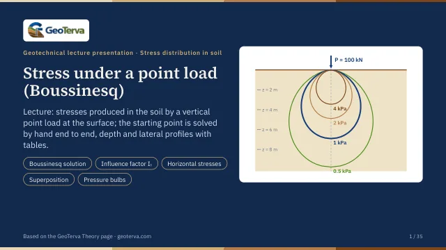
Lecture slides
Ready-made slides for lectures and self-study
The mechanism, the derivation, the equations and the figures of this page, in teaching order. Every slide links back to its chapter.
1Scope and assumptionsBoussinesq’s half-space.
Boussinesq (1883) solved the stresses produced at any point of a homogeneous, elastic and isotropic medium by a point load on the surface of an infinitely large half-space. The solution is the basis of every other load in this program: a line, strip, circular or rectangular load is a sum of point loads. Its assumptions:
- The soil is a semi-infinite medium: it extends without limit sideways and downward below a plane surface.
- It is homogeneous, isotropic and linearly elastic, with Poisson’s ratio μ; the modulus of elasticity does not appear in the stresses.
- The load P is a vertical point load on the surface. The stresses found are increases caused by the load; the stresses already in the ground from its own weight are added to them.
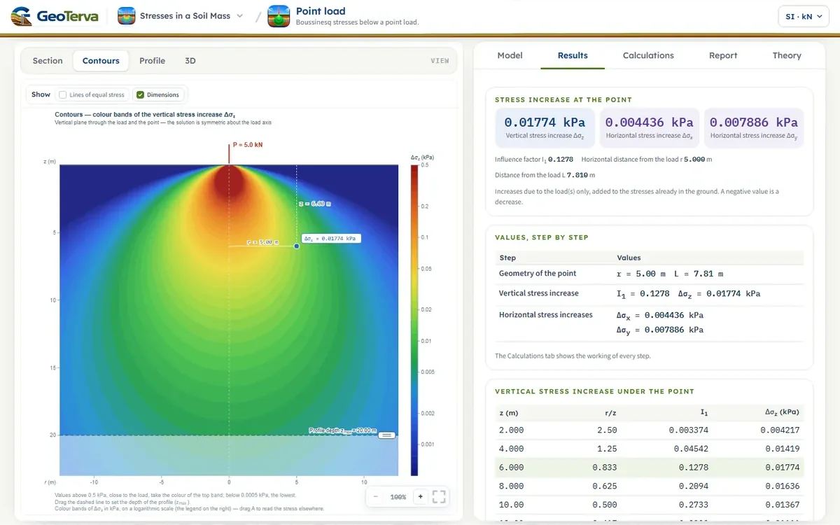
The module gives the vertical stress increase Δσz and the horizontal ones Δσx, Δσy at the point, and Δσz against depth under it.
2Boussinesq’s solutionThe three normal stresses at a point.
With the coordinates of the figure, the normal stresses at the point are
The horizontal stresses depend on Poisson’s ratio μ; the vertical stress does not — nor on the modulus of elasticity. For μ = 0.5 (no volume change, undrained clay) the brackets vanish and Δσx = 3P x²z/(2πL⁵), Δσy = 3P y²z/(2πL⁵). On the load axis (r = 0) both horizontal stresses tend to −P(1 − 2μ)/(4π z²), a small decrease.
Several point loads. In a linearly elastic soil the stresses of separate loads add (superposition). For loads Pk at (xL,k, yL,k) each is taken alone with the point at (x − xL,k, y − yL,k) from it, so that rk and Lk are its own, and Δσz = ΣΔσz,k, Δσx = ΣΔσx,k, Δσy = ΣΔσy,k. The module takes up to eight loads, no two at the same position; the lines of equal stress of the Section view are then drawn in the vertical plane y = yA through the point, parallel to x, and a load beside that plane acts on it all the same.
3The influence factor I1Δσz = (P/z²) I1.
Since L² = z²[(r/z)² + 1], the equation can be written with a factor that depends on r/z alone:
| r/z | I1 | r/z | I1 |
|---|---|---|---|
| 0.0 | 0.4775 | 0.1 | 0.4657 |
| 0.2 | 0.4329 | 0.3 | 0.3849 |
| 0.4 | 0.3295 | 0.5 | 0.2733 |
| 0.6 | 0.2214 | 0.7 | 0.1762 |
| 0.8 | 0.1386 | 0.9 | 0.1083 |
| 1.0 | 0.0844 | 1.2 | 0.0513 |
| 1.4 | 0.0317 | 1.6 | 0.0200 |
| 1.8 | 0.0129 | 2.0 | 0.0085 |
| 2.5 | 0.0034 | 3.0 | 0.0015 |
| 4.0 | 0.0004 | 5.0 | 0.0001 |
4Lines of equal stressThe pressure bulbs of a point load.
Joining the points of equal Δσz gives the bulb-shaped lines of the figure (the Section view draws them for the entered load). Along the load axis the stress falls with the square of the depth, Δσz = 0.4775 P/z²; at a given depth it falls quickly away from the axis. Close to the load the solution gives very large stresses — a real load is never a point, and near it the Profile view marks the stress as growing beyond the axis.
5Worked examplesEvery number computed by the module’s own code.
First example — depth profile
P = 5 kN; the point x = 3 m, y = 4 m, so r = 5 m; Δσz at z = 2, 4, 6, 10 and 20 m:
| z (m) | r/z | I1 | Δσz (kPa) |
|---|---|---|---|
| 2 | 2.500 | 0.0034 | 0.0042 |
| 4 | 1.250 | 0.0454 | 0.0142 |
| 6 | 0.833 | 0.1278 | 0.0177 |
| 10 | 0.500 | 0.2733 | 0.0137 |
| 20 | 0.250 | 0.4103 | 0.0051 |
Second example — along a line
The same load; z = 2 m, y = 3 m and x = 0 to 4 m:
| x (m) | r (m) | r/z | I1 | Δσz (kPa) |
|---|---|---|---|---|
| 0 | 3.00 | 1.500 | 0.0251 | 0.0313 |
| 1 | 3.16 | 1.581 | 0.0208 | 0.0260 |
| 2 | 3.61 | 1.803 | 0.0128 | 0.0160 |
| 3 | 4.24 | 2.121 | 0.0067 | 0.0084 |
| 4 | 5.00 | 2.500 | 0.0034 | 0.0042 |
The module opens with the first example at z = 6 m.
6ReferencesSources.
- Boussinesq, J. (1883). Application des Potentiels à l’Étude de l’Équilibre et du Mouvement des Solides Élastiques. Gauthier-Villars, Paris.
- Das, B.M. (2018). Principles of Geotechnical Engineering, 9th ed. Cengage Learning.
From theory to your own design
Find the stress below your own point loads in minutes
- The vertical and the horizontal stress increases at any point, with Poisson's ratio
- Several point loads in one model
- The depth profile, the lines of equal stress and the 3D view
- A clean calculation report, saved as a PDF. Online: nothing to install, no dongle, on a phone, a tablet or a PC