
On this page · 7 chapters
The active force on a wall during an earthquake by the pseudo-static method: Mononobe–Okabe for a granular backfill with wall friction, an inclined back and a sloping surface, the line of action after Seed & Whitman (1970), and the module’s layered form with a water table and a surcharge.
 PDF
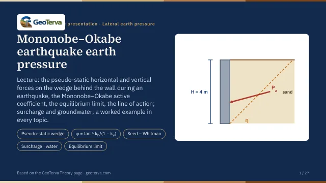
Lecture slides
Ready-made slides for lectures and self-study
The mechanism, the derivation, the equations and the figures of this page, in teaching order. Every slide links back to its chapter.
1The pseudo-static wedgeCoulomb's wedge with kₕW and kᵥW.
During an earthquake the soil wedge behind a wall is accelerated. The pseudo-static method replaces the shaking by two constant body forces on Coulomb's trial wedge ABC (Okabe 1926; Mononobe & Matsuo 1929):
- kₕW — horizontal, toward the wall, with kₕ = horizontal acceleration / g;
- kᵥW — vertical, with kᵥ = vertical acceleration / g (taken upward here, so it reduces the weight);
- W, F (at φ′ to the normal of BC) and Pₐₑ (at δ′ to the normal of the back) as in Coulomb's analysis.
W, kₕW and kᵥW add up to a force W(1 − kᵥ)/cos ψ, tilted from the vertical by the seismic angle
so the seismic wedge is Coulomb's wedge in a gravity field turned by ψ: the wall back becomes θ + ψ and the backfill α + ψ. As in Coulomb's analysis, the dynamic active force is the largest of the trial-wedge forces.
2Mononobe–Okabe coefficientThe dynamic active force.
Maximising the trial-wedge force gives the Mononobe–Okabe equations:
With kₕ = kᵥ = 0, ψ = 0 and K′ₐ is Coulomb's Kₐ. The coefficient grows quickly with kₕ and without bound as the equilibrium limit is approached:
| kₕ | φ′ = 28° | φ′ = 30° | φ′ = 35° | φ′ = 40° | φ′ = 45° |
|---|---|---|---|---|---|
| 0.1 | 0.396 | 0.368 | 0.306 | 0.253 | 0.207 |
| 0.2 | 0.485 | 0.452 | 0.380 | 0.319 | 0.267 |
| 0.3 | 0.604 | 0.563 | 0.474 | 0.402 | 0.340 |
| 0.4 | 0.778 | 0.718 | 0.599 | 0.508 | 0.433 |
| 0.5 | 1.115 | 0.972 | 0.774 | 0.648 | 0.552 |
3The limit of equilibriumThe critical horizontal acceleration.
The term sin(φ′ − α − ψ) under the root has no real value when φ′ − α − ψ < 0: no wedge can then be in equilibrium, whatever the wall does. The backfill is stable only while
For a level backfill this is ψ ≤ φ′, i.e. the horizontal acceleration may not exceed
(for a sloping backfill, tan(φ′ − α) in place of tan φ′). The module stops with a message when kₕ is above this limit; near it K′ₐ rises steeply (Figure 2).
4Line of actionSeed & Whitman.
The Mononobe–Okabe analysis gives the size and direction of Pₐₑ but not where it acts. Seed & Whitman (1970) split it into the static Coulomb force and a seismic increment:
Pₐ (Coulomb, ½γH²Kₐ with the same δ′, θ, α) acts at H/3 above the base; ΔPₐₑ acts higher, at 0.6H. The resultant acts at
still inclined at δ′ to the normal of the back.
5Layers, water and surchargeA layered backfill with a water table and a surcharge (this module).
A surcharge q on the backfill surface (vertical, per unit area of the sloping surface) adds its weight to every trial wedge in the same proportion as the soil, and in the earthquake its inertia with it, so the critical wedge does not change. As for Coulomb’s force it acts as the vertical stress
The module also takes the backfill in layers, their boundaries level and their thicknesses measured vertically at the back from its top A, each with its own γ, φ′ and wall friction δ′. Each layer takes its own coefficient under the effective vertical stress below A:
per unit length of the back, inclined at the δ′ of the layer to its normal. A level water table at zw below A, with hydrostatic pore pressure, makes the layers weigh γ′ = γsat − γw below it, and u = γw(z − zw) acts normal to the back. In the earthquake the pore water either moves with the soil — restrained, the usual case for a backfill of low permeability — or, in a highly permeable backfill (k > 5×10⁻⁴ m/s), does not — free. The inertia is then that of the saturated or of the dry mass, while the buoyant weight carries the stress, and the seismic angle below the water table grows:
Free water adds its own hydrodynamic pressure, after Westergaard (1933), over the height dw of the water table above the base:
For the line of action the static Coulomb part (the same layers with kₕ = kᵥ = 0) acts where its pressures put it and the seismic increment ΔN = Nae − Na at 0.6H, as Seed & Whitman do for one soil; the water and its hydrodynamic pressure act with their own arms. The increment is sometimes taken at mid-height; the module keeps the 0.6H of Seed & Whitman, which gives the larger overturning moment.
The Mononobe–Okabe wedge is a single plane through one dry soil; the layered form is the module’s engineering extension of it, not a closed-form layered solution of the literature. For one dry soil it reduces to the closed form of Mononobe–Okabe; with kₕ = kᵥ = 0 it is the layered Coulomb solution of the Coulomb module. The critical plane of each layer, drawn from the heel through the layers, is a piecewise approximation of the mechanism.
6Worked exampleThe wall the module opens with.
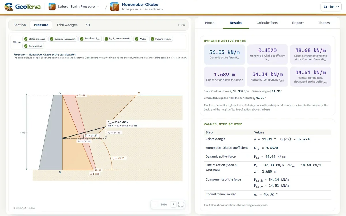
A wall H = 4 m with γ = 15.5 kN/m³, φ′ = 30°, δ′ = 15°, θ = α = 0, kᵥ = 0 and kₕ = 0.2. Find Pₐₑ and its line of action.
The module opens with this example.
7ReferencesSources.
- Das, B.M. (2018). Principles of Geotechnical Engineering, 9th ed. Cengage Learning.
- Mononobe, N. and Matsuo, H. (1929). On the determination of earth pressure during earthquakes. Proceedings, World Engineering Congress, Tokyo, 9, 177–185.
- Okabe, S. (1926). General theory of earth pressure. Journal of the Japan Society of Civil Engineering, 12(1).
- Seed, H.B. and Whitman, R.V. (1970). Design of earth retaining structures for dynamic loads. Specialty Conference on Lateral Stresses in the Ground and Design of Earth Retaining Structures, ASCE, 103–147.
- Das, B.M. (2016). Principles of Foundation Engineering, 8th ed. Cengage Learning.
- Westergaard, H.M. (1933). Water pressures on dams during earthquakes. Transactions ASCE, 98, 418–433.
From theory to your own design
Find the seismic force on your own wall in minutes
- The dynamic active force, its components and its line of action, step by step
- The horizontal and the vertical seismic coefficients, an inclined back and a sloping backfill
- Layers, a water table and a surcharge
- A clean calculation report, saved as a PDF. Works on your phone and in your browser