
On this page · 19 chapters
- 1Sheet-pile walls and this module
- 2How a cantilever wall moves
- 3Active pressure above the dredge line
- 4The net pressure below the dredge line
- 5Equilibrium: the embedment equation
- 6The depth of embedment
- 7The maximum bending moment
- 8No water table
- 9Water at different levels on the two faces
- 10Verifying the sheet pile to EN 1993-1-1
- 11Verifying the sheet pile to AISC 360-22
- 12The sloping retained surface
- 13The anchored wall
- 14The seismic situation
- 15The displacement of the wall
- 16A worked example, by the module
- 17The opening wall, verified to EN 1993-1-1
- 18What the module assumes
- 19References
A cantilever sheet-pile wall holds itself up by the passive resistance of the sand it is driven into. This page follows the source, section by section — how the wall moves, the net pressure diagram, the embedment equation, the depth of embedment and the maximum moment — and then the verification of the sheet pile to EN 1993-1-1 or AISC 360-22, with a worked example and the opening wall computed by the module's own code.
 PDF
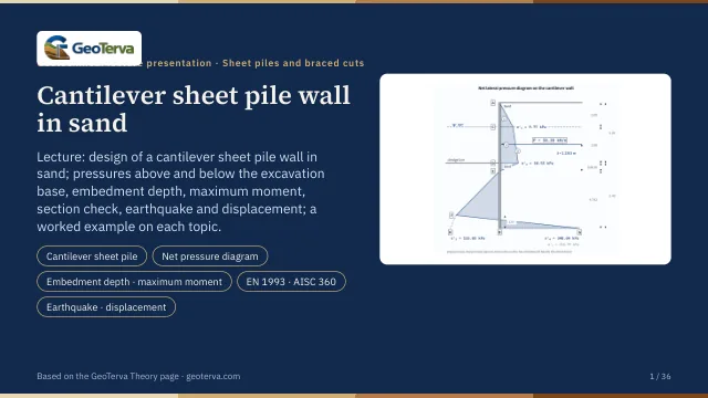
Lecture slides
Ready-made slides for lectures and self-study
The mechanism, the derivation, the equations and the figures of this page, in teaching order. Every slide links back to its chapter.
1Sheet-pile walls and this modulewhat a sheet-pile wall is, and which one is designed here
A sheet-pile wall is a row of interlocking piles driven into the ground to retain soil or water — a waterfront quay, a cofferdam, the side of an excavation. Timber, precast concrete and steel have all been used; steel sections dominate because they are light to handle, drive well and are re-usable. The steel piles come in two shapes, the Z-section and the U-section, and a manufacturer's table gives each one's section modulus per metre of wall — the number a design ends up looking the table up with.
Two ways of building the wall lead to the same structure: in a backfilled structure the piles are driven first and the soil is placed behind them; in a dredged structure the piles are driven into the existing ground and the soil in front of them is then removed down to the dredge line. Either way the wall ends up retaining a height L of soil above the dredge line, and holding itself up by its embedment D below it (the figure below).
A cantilever wall has no other support: it stands like a fence post, fixed only by the passive resistance of the soil it is driven into. That makes it economical for moderate heights — as a rule up to about 6 m above the dredge line — beyond which an anchored wall, tied back near its top, is used instead.
This module designs a cantilever wall driven into sand: sand layers down the whole profile — above the dredge line they are retained, below it they act on both faces of the wall — and a water table standing at the same level on both faces (the source's case) or at different levels (the net water pressure added). A cantilever wall in clay is its own module.
2How a cantilever wall movesrotation about a point near the toe, and the three zones of pressure
Under the push of the retained soil the wall rotates as a rigid body about a point O a little above its toe (the figure below). The rotation sets the pressures:
- Zone A, above the dredge line: only the retained soil is there, pushing with its active pressure.
- Zone B, from the dredge line down to O: the wall moves toward the excavation, so the retained side is active and the soil in front, being pushed, resists with its passive pressure.
- Zone C, below O: the wall moves the other way, and the sides swap — passive behind, active in front.
The true distribution is curved. The source replaces it with a straight-line construction: the net pressure below the dredge line falls on one straight line through a zero point E — a point of the diagram, not the rotation point O — and the reversal at the toe is drawn as a block of height . Horizontal and moment equilibrium of that diagram fix the embedment.
3Active pressure above the dredge lineσ′₁ at the water table, σ′₂ at the dredge line
Above the dredge line only the retained sand acts, with its Rankine active pressure — the effective overburden times the active coefficient. No wall friction is credited.
With the water table a depth below the top of the wall and the rest submerged, the pressure at the water table and at the dredge line are
The water stands at the same level on both faces of the wall, so the hydrostatic pressures on the two sides cancel and only these effective pressures load it.
A uniform surcharge spread over the whole retained surface — traffic, stored material — adds to the effective overburden at every depth on the retained side. The active diagram then starts from at the top of the wall, and every ordinate below gains :
A load of limited extent — a strip parallel to the wall or a point load — does not add a constant . Its lateral pressure is taken from the elastic half-space, doubled for a rigid, unyielding wall by the image method:
where is the angle the strip subtends at the depth and the angle of its bisector from the vertical; the point load is taken on the section of wall through it — the most loaded metre — and used for the whole wall. These pressures are added to the retained face down the whole wall, above and below the dredge line; the net diagram is then curved and the module integrates it numerically.
Below the dredge line the same stays in the overburden of the retained side, so the net line starts from the larger and the passive pressure of the retained side at the toe grows by ; the excavation side carries none of it. The rest of the construction is unchanged.
4The net pressure below the dredge linethe straight line through the zero point E
Below the dredge line both faces have soil against them. The retained side keeps pushing actively, the excavation side resists passively, and the passive pressure grows faster with depth. The net pressure therefore starts at just below the dredge line and falls linearly with depth:
It reaches zero at the point E, a depth below the dredge line:
5Equilibrium: the embedment equationP and z̄, the toe block, and the fourth-degree equation in L₄
Above E the diagram pushes the wall toward the excavation with a resultant P, acting a height above E — the area of the active diagram and of the triangle between the dredge line and E, and its centroid. Below E the net line continues, now as the reversed passive resistance, and at the toe the pressure swings back over the height . Two conditions close the diagram:
With the depth of the toe below E, the ordinates of the construction are
and eliminating between the two conditions leaves one equation of the fourth degree in :
6The depth of embedmentDtheory, and the two ways of adding a margin
The theoretical embedment is the depth at which the diagram is exactly in equilibrium:
At that depth the passive resistance is fully mobilised and there is no margin at all. The source offers two ways of adding one (the figure below):
- Increase the depth: the diagram is built with the full and the depth is increased by 20 to 30 percent, with to . The pressures and the moment are those of the theoretical wall.
- A factor of safety on Kp: the diagram is built from the start with , to , and the depth that comes out is used as it is. Every ordinate below the dredge line changes, and the moment grows with them.
A depth of your own. Instead of taking the design depth from the analysis, the depth of the sheet pile below the dredge line may be given. It is then verified against the depth the chosen route requires, and the factor of safety it mobilises on the passive coefficient is found — the factor by which can be divided before the diagram is only just in equilibrium at the given depth:
The total length, the displacement and the seismic check are worked with the given depth. For the internal forces two cases are worked: the required-depth design case, and the given-depth equilibrium case with the passive coefficient divided by . The moment of the design case is not an upper bound of the given one — a longer wall in equilibrium with a partly mobilised passive resistance can bend more — so the sheet pile and the anchors are designed for the larger of the two; in the seismic situation the same is done when the given depth exceeds . The uniform mobilisation of is itself an idealisation.
7The maximum bending momentzero shear at z′ below E, and Mmax there
The bending moment is largest where the shear is zero. Below E the net passive triangle grows as ; it has cancelled P a depth below E:
8No water tablethe same diagram with the moist unit weight
Without a water table the same construction holds with the moist unit weight throughout: the active pressure at the dredge line and the zero point become
and every of the equations above becomes . The embedment equation keeps its form.
9Water at different levels on the two facesthe net water pressure added (beyond the source)
The source assumes the water stands at the same level on both faces. A dewatered excavation, or standing water in front of the wall, breaks that assumption: the hydrostatic pressures no longer cancel.
The module then adds the net water pressure to the net effective pressure for the no-seepage hydraulic condition, and gives each face its own effective overburden:
The net line is then piecewise, so its zero point, the resultant above it and the two equilibrium equations are solved on the diagram itself rather than by the closed form; the construction — zero point E, toe block — is the same.
10Verifying the sheet pile to EN 1993-1-1from S = M/σall to MEd ≤ W fy / γM0
The classical route sizes the pile with an allowable stress:
The module replaces it with a limit-state verification. The moment of the net-pressure diagram is a characteristic action effect; the partial factor raises it to a design value, and EN 1993-1-1 compares the design moment with the resistance of the section:
is the number to look the sheet-pile table up with. The pile given is then checked against it. The table prints two moduli per size, and the class of the section decides which may be used (the figure below): the elastic holds the section to first yield and is valid up to class 3; the plastic lets it reach its full plastic moment, which is allowed for a class 1 or 2 section.
| Factor | what it acts on | value |
|---|---|---|
| the earth-pressure moment, a permanent unfavourable action | 1.35 | |
| the resistance of a cross-section | 1.00 |
11Verifying the sheet pile to AISC 360-22LRFD or ASD on the flexural strength Mn
The pile may instead be verified to AISC 360-22. Its nominal flexural strength is for a compact section — the plastic modulus — or at first yield, and it is compared with the moment by one of two methods:
The earth pressure is taken as the lateral earth pressure H: in the LRFD combinations it enters with where it adds to the load effect, in the ASD combinations with 1.0.
12The sloping retained surfacean infinite slope behind the wall — Rankine for a sloping backfill
When the ground behind the wall rises at an angle and keeps rising, the retained soil is no longer in the Rankine state of a level surface. For a cohesionless soil under an infinite slope Rankine's solution gives an active pressure that acts parallel to the slope, proportional to the vertical depth below the surface at the wall:
At it is ; it has no solution once — a sand does not stand steeper than its friction angle. The wall takes the horizontal part, , and the module uses it in place of on the retained side, above and below the dredge line; the vertical part, a friction on the wall, is not credited. The excavation side stays level. The passive coefficient of the retained side at the toe — the reversal of a cantilever — is kept level: the slope would raise it, so the level value is on the safe side.
The same state is the planar wedge of Coulomb with the wall friction . Its critical plane, found by searching the plane angle, rises from the dredge line at ; the bond zones of the anchors are placed behind that plane with a margin. In the seismic situation the retained side takes the Mononobe–Okabe coefficient of the slope with , which reduces to at and has no solution when :
In the displacement model the retained side starts from the at-rest pressure of the slope, , and its active limit is .
13The anchored wallone row or several — free earth support, the hinge idealisation, the anchor reactions and the bond zones
Where the cantilever grows too long or bends too much, a row of anchors near the top of the wall holds it back. With one row the source designs the wall by the free earth support method: the anchor is a support at the depth , and the embedment is only deep enough for the passive resistance to balance the moments about it — the toe is free to move, so there is no reversal of pressure at the toe.
The net pressure is the same diagram as for the cantilever — active above the zero point E, net passive below it — cut off at the toe. The first equation fixes the depth, the second the anchor force per metre of wall; over the spacing and along the tendon axis it is the support reaction of each anchor. is a reaction of the design diagram — not the lock-off load and not the force the tendon carries in service; the prestressed spring model of the displacement gives its own tendon force , and the tendon resistance and the bond capacity are separate checks. The moment peaks where the shear below the anchor, , is zero. For one sand the first equation is the cubic in ; the module solves it numerically, so layers, water, surcharge and the seismic situation all follow.
Several rows. With more than one row the wall is statically indeterminate. The module makes it determinate with the structural idealisation of the hinge method: a hinge is put at every anchor below the uppermost, so that the wall between two anchors is a simple beam, and the part below the lowest anchor is designed by free earth support about it. The depth comes from the moments about the lowest anchor, each span gives the reactions at its two anchors, and the anchor force of a row is the sum of the reactions it receives:
The uppermost span also carries the cantilever above the first anchor. The module applies the idealisation to its limit-equilibrium net-pressure diagram, so the reactions and the moments are those of that diagram. With one row the method is exactly the free earth support method. The moment peaks at the zeros of the shear between and below the anchors, or at the uppermost anchor. The anchors pull the wall down by each; that vertical component is reported, not carried into the check of the sheet pile.
The anchor holds the wall only if its bond zone lies in soil that stays in place when the active wedge moves. the module takes an unbonded length of at least 4.5 m (strand tendons; 3 m for bars) and the bond zone to start at least behind the critical failure surface — for a cohesionless soil the Rankine plane rising from the dredge line at :
In the displacement model the anchor is a prestressed spring: it starts with per metre of wall and stiffens with , the free length stretching as the wall moves.
14The seismic situationpseudo-static Mononobe–Okabe coefficients, restrained water, Westergaard
In an earthquake the soil behind the wall and in front of it is shaken with it. The pseudo-static method replaces the shaking by constant inertia forces on the soil wedges — horizontally and vertically — and keeps the limit-equilibrium construction of the static design. The engineer gives and from the governing seismic code; a common form is and .
Rotating the gravity of the wedge by the angle θ turns Coulomb's wedge into that of Mononobe and Okabe. For a vertical wall, a level surface and no wall friction — the same idealisation as the static Rankine design — the coefficients are
At they are exactly and . The pressures are and ; both senses of are checked. With wall friction the Mononobe–Okabe passive coefficient becomes unsafe, which is why the log-spiral solutions exist; with it is not, and the plane wedge is kept. When there is no wedge in equilibrium at all and the module says so.
Water. A sand of ordinary permeability is dynamically impervious: its pore water moves with it. Below the water level the submerged unit weight carries the pressure while the inertia acts on the saturated mass, so the angle grows:
In a highly permeable soil ( m/s) the pore water is free instead (Annex E.7): only the dry mass carries inertia, , with the dry unit weight entered for each layer. The pore water of each face is then one free column from its water level down to the base of the wall, and adds the Westergaard pressure with measured from the base, as E.7 measures it; the two faces shake in phase, one pressed and the other sucked, so their pressures act together toward the excavation. Carrying E.7 down the embedded part of a sheet pile is an extension of this module. The module offers both.
Water standing free in the excavation above the dredge line adds the hydrodynamic pressure of Westergaard (1933), taken in the unfavourable sense, as a suction on the excavation face:
The check. The net-pressure diagram is built with these coefficients exactly as the static one — the same layers, water and surcharge, the zero point E and the toe block — and its two equilibrium equations give the embedment . The seismic situation is accidental, so carries no factor: the wall as designed holds if . For a cantilever the seismic pressures are distributed like the static ones, in proportion to the effective overburden: it is free to rotate about its toe, and the dynamic increment then acts at the point of the static thrust.
The anchored wall cannot rotate about its toe, and for such a wall the dynamic increment acts at mid-height. The retained side keeps its static Rankine pressure above the dredge line, and the increment of the active thrust over the retained height is spread uniformly over it:
Below the dredge line the Mononobe–Okabe coefficients act on the overburden. The same anchored construction then gives and the seismic anchor forces . The active wedge of the earthquake is flatter than the static one — its plane rises at the Mononobe–Okabe angle , at — and the bond zones are checked behind it with the same margin; the tendon and the bond are not verified for .
The sheet pile is then verified under the seismic combination: in the seismic design situation the permanent actions and the seismic action enter with 1.0 and the variable ones with — each surcharge takes the entered with it, 1.0 for a permanent load — so of that diagram; in the LRFD and ASD routes the earth pressure H keeps 1.6 (LRFD) or 1.0 (ASD) and the seismic rise E enters with 1.0 or 0.7, and , the two maxima combined on the safe side.
The opening wall with and — the water standing 2 m below the top on both sides, so 3 m of free water in the excavation:
The static design would not hold in this earthquake: the seismic diagram needs a toe 2.96 m deeper and 3.0 times the static moment.
15The displacement of the wallthe subgrade reaction method: an elastic beam on elasto-plastic springs
The limit-equilibrium construction of the previous sections gives the depth of embedment and the design moment, but not how far the wall moves: it describes the wall at the moment of failure, with the passive resistance fully mobilised. To estimate the displacement under working conditions the module uses the subgrade reaction method — a Winkler model, in which the wall is an elastic beam and the soil on each face a row of independent springs.
Here is the displacement of the wall toward the excavation, its bending stiffness per metre of wall, and , the effective pressures of the retained and the excavation side. Each spring starts from the pressure at rest and changes in proportion to the displacement, never beyond the active or the passive pressure:
The coefficient of horizontal subgrade reaction is the pressure per unit displacement. It is a parameter of the model rather than a property of the soil — it depends on the wall and on the loaded height as well — and the displacement depends on it: strongly while the springs are soft, hardly at all once the soil on both faces has reached its active and passive pressures, so the result is an estimate. For orientation, typical values for sand are: loose 4.8–16, medium dense 9.6–80, dense 64–128 MN/m³.
- The wall has its design length, , and both of its ends are free.
- The pressures are characteristic: the full Rankine , no factor of safety; the at-rest coefficient is that of Jaky (1944).
- The wall is in place before the excavation, which is made in one stage; the construction sequence is not followed.
- The equation is solved by beam finite elements, the springs iterated until each is either elastic or at its active or passive limit.
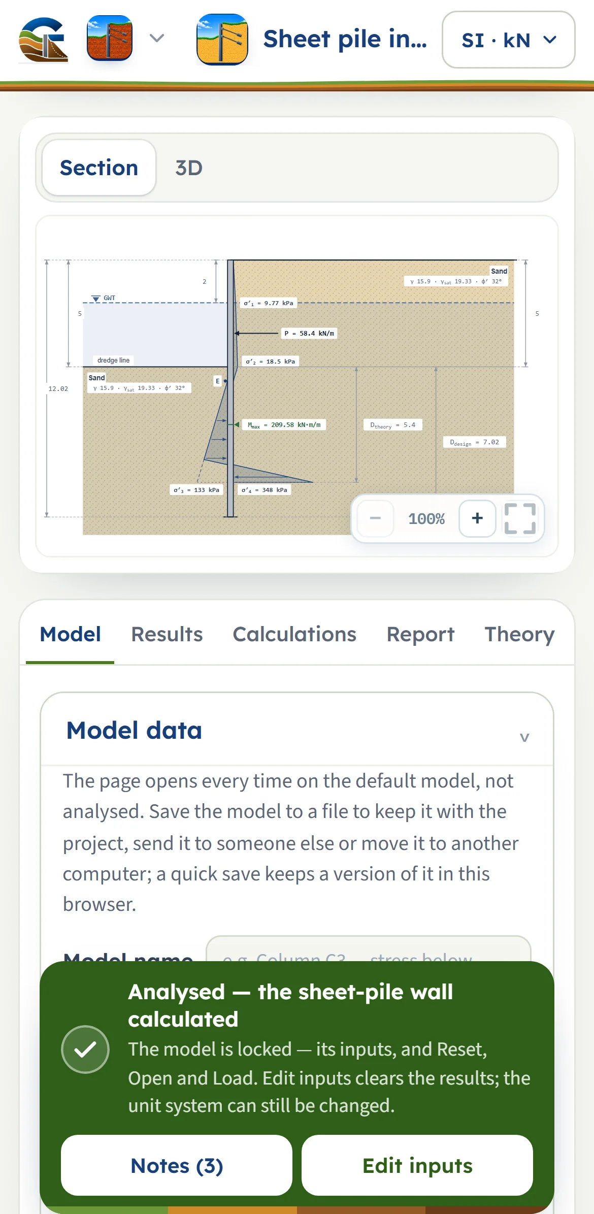
The opening wall, with the design length 12.02 m, = 21000 cm⁴/m, = 210 000 MPa and = 20 MN/m³:
The largest moment of this model, 209.58 kN·m/m, is that of the limit-equilibrium construction (209.58 kN·m/m): the retained side is at its active pressure and the soil in front at its passive pressure over the whole height where the moment builds up.
16A worked example, by the moduleevery number computed by the module's own code
The worked example is a cantilever wall retaining L = 5 m of sand (γ = 15.9 kN/m³, γsat = 19.33 kN/m³, φ′ = 32°) above the dredge line, the water table 2 m below the top on both sides, driven into the same sand; the depth increased by 30 percent. Run through the module's own calculation:
| Quantity | module |
|---|---|
| (kPa) | 18.55 |
| (m) | 0.66 |
| (kN/m) | 58.38 |
| (m) | 2.23 |
| (m) | 4.74 |
| (m) | 5.40 |
| (kN·m/m) | 209.58 |
| (cm³/m), σall = 172 MPa | 1218 |
17The opening wall, verified to EN 1993-1-1MEd, Wreq, Mc,Rd and η for the default model
The wall the Model tab opens with is the wall of the worked example above, with a sheet pile of steel S275 given by its elastic modulus Wel = 1400 cm³/m, verified to EN 1993-1-1 with and :
The pile carries the design moment. The Calculations tab writes out the same chain for whatever wall is entered.
18What the module assumesthe limits of the calculation, in one place
- Rankine pressures without wall friction, on the effective overburden; the profile is sand from top to bottom, in any number of layers (a clay embedment is its own module). One sand below the dredge line keeps the closed form of the source; several are solved on the same diagram numerically.
- The source's simplified net-pressure diagram: one straight line through the zero point E and a toe block; the rotation point is not located more exactly.
- Water at the same level on both faces, or at different levels with the no-seepage condition; seepage and its effect on the passive resistance are not modelled.
- The depth of embedment carries the margin of its own route — the depth factor f or FSp on Kp — and is not factored again by the steel code.
- The sheet pile is verified in bending on the modulus given, taken as that of the whole wall; the shear of the wall, local buckling of its elements and corrosion loss are not verified.
- The displacement of the wall is estimated by the subgrade reaction method with characteristic pressures and reported without a limit; the settlement behind the wall is not computed. A cantilever wall is rarely economical beyond D ≈ 1.5–2 L, and the module notes a theoretical embedment deeper than 3 L.
19Referencesthe sources
- Das, B.M. (2016). Principles of Foundation Engineering, 8th ed. Cengage Learning.
- EN 1993-1-1:2005 — Design of steel structures, general rules.
- ANSI/AISC 360-22 — Specification for Structural Steel Buildings.
- Bowles, J.E. (1996). Foundation Analysis and Design, 5th ed. McGraw-Hill.
- Jaky, J. (1944). The coefficient of earth pressure at rest. Journal of the Society of Hungarian Architects and Engineers, 7, 355–358.
- Mononobe, N. and Matsuo, H. (1929). On the determination of earth pressure during earthquakes. World Engineering Congress, Tokyo. Okabe, S. (1926). General theory of earth pressure. Journal of the Japan Society of Civil Engineering, 12(1).
- Westergaard, H.M. (1933). Water pressures on dams during earthquakes. Transactions of the American Society of Civil Engineers, 98, 418–433.
From theory to your own design
Design your own sheet-pile wall in minutes
- The net pressure diagram, the embedment depth and the maximum moment, step by step
- Water on both faces, a surcharge, a sloping surface and the earthquake
- The sheet pile checked to EN 1993-1-1 or AISC 360-22
- A clean calculation report, saved as a PDF. Works on your phone and in your browser