
On this page · 6 chapters
The horizontal pressure that rectangular area loads on the ground add to a vertical wall, by Boussinesq integration: the stress of a point load, the closed form along the wall, the rigid wall and the half-space, the shear force and the bending moment. The figures and every number are computed from the module's own equations.
 PDF
Lecture slides
Ready-made slides for lectures and self-study
The mechanism, the derivation, the equations and the figures of this page, in teaching order. Every slide links back to its chapter.
1Area loads on a wallWhat the module computes.
A rectangular surface surcharge is a continuous field of vertical point loads dP = q·dA. The horizontal stress each of them produces on a chosen vertical section of the wall follows from the elastic half-space solution of Boussinesq, and the contributions of every rectangle are added. The resulting lateral-pressure profile is integrated down the wall to give the shear force and the bending moment.
Geometry of an area load
- — uniform vertical surcharge over the rectangle
- — centroid coordinate perpendicular to the wall
- — centroid coordinate along the wall
- — rectangle side perpendicular to the wall
- — rectangle side along the wall
- — along-wall coordinate of the section evaluated
Relative to the section, a rectangle occupies x from x₁ to x₂ and y from y₁ to y₂, and it must lie behind the wall face, x₁ ≥ 0:
2Stress from a point loadBoussinesq σx on the plane of the wall.
For an element dP at the plan offset (x, y) from a point of the section at the depth z, with r² = x² + y² and R² = r² + z², the horizontal normal stress perpendicular to the wall is
3Integrating a rectangleClosed form along the wall; rigid wall or half-space.
Replacing the rectangle by a finite grid of point loads converges slowly near the wall, where the stress changes fastest. The integral along the wall has a closed form: with a² = x² + z², the function
The remaining integral across the wall is evaluated adaptively to a tight tolerance. A very long rectangle recovers the plane-strain strip load exactly, whatever μ, which is one of the checks the engine is tested against.
Rigid wall or half-space
A smooth wall that does not move is represented by mirroring every load across the wall face: the image cancels the wall-normal displacement and the shear on that plane, so the pressure on the wall is exactly twice the half-space stress, for any μ. A wall that deflects enough to relieve the soil is closer to the half-space value:
4Shear force and bending momentThe profile integrated down the wall.
The pressure profile is integrated down the wall once for the shear force and twice for the bending moment, per unit length of wall at the section:
Both are integrated adaptively between the rows of the depth table; the number of rows nz only sets how much of the profile is listed.
5Worked exampleThe sequence by hand and the default example.
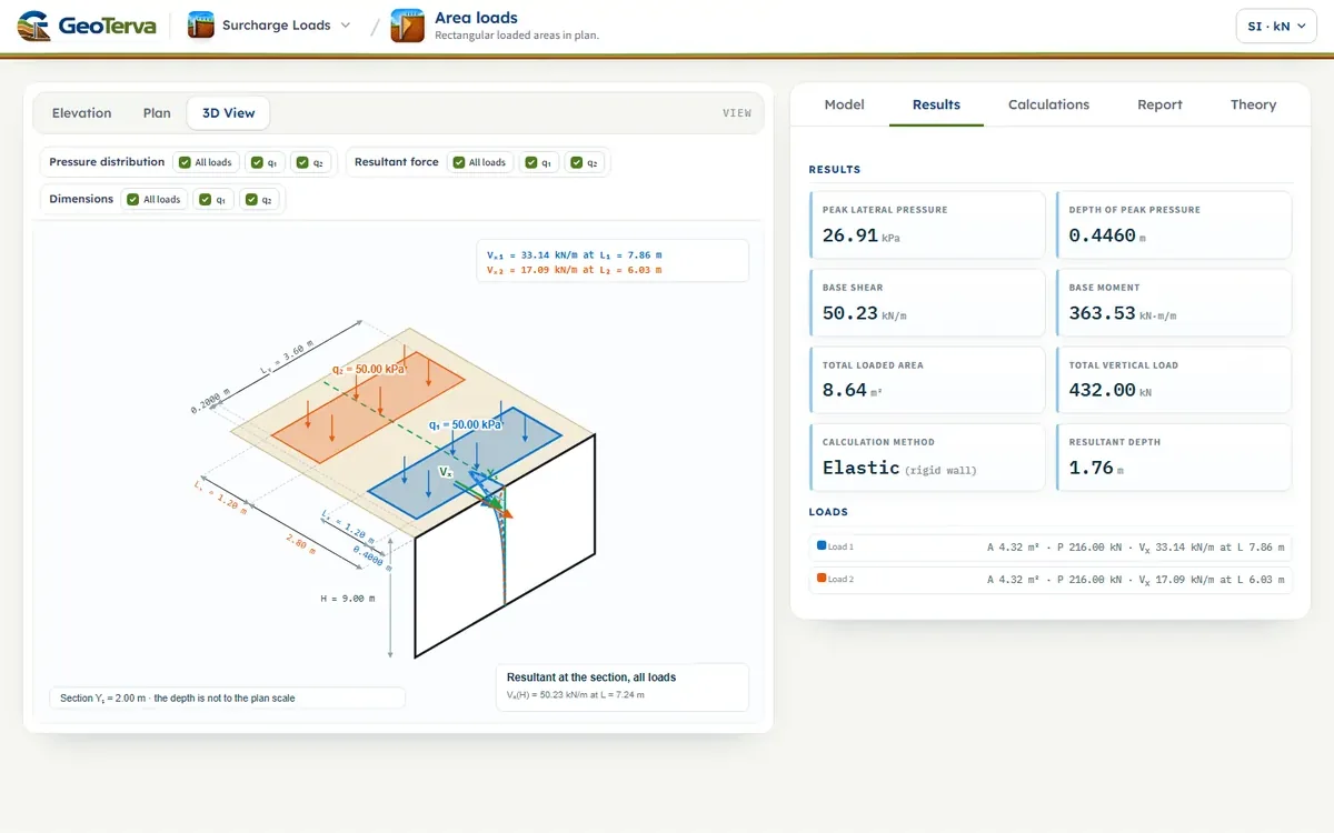
The data are H = 9.00 m, μ = 0.50, Ys = 2.00 m and two rectangles of 1.2 × 3.6 m with q = 50 kPa at X₀ = 1.0 m and 3.4 m, Y₀ = 2.0 m; the example is fixed and does not follow the inputs of the interface. By hand, the sequence is:
- Define the wall and the section: enter H, μ and the section coordinate Ys.
- Define each rectangle: enter q, X₀, Y₀, Lx and Ly; find x₁, x₂, y₁, y₂ (Eq. (2), Eq. (3)).
- Point-load stress: for dP = q·dx·dy evaluate r, R and σx (Eq. (4)).
- Integrate the area: exactly in y with G, numerically in x (Eq. (5)).
- Superimpose and apply ψ: add every rectangle at the depth z; double for a rigid wall (Eq. (6)).
- Integrate down the wall: build σx(z), then Vx(z) and My(z) (Eq. (8), Eq. (9)).
Totals and the peak pressure
The wall base
Engineering interpretation
The method keeps the three-dimensional position and size of every load: moving a rectangle along the wall, away from it, resizing it, moving the section or changing μ all change the pressure profile. The pressure peaks on sections that pass in front of a load and decays quickly with the plan distance, so several sections should be checked when loads are short compared with their distance from the wall. With μ below 0.5 small tension ordinates can appear near the surface; they are reported with their sign.
6ReferencesSources.
- Das, B.M. (2016). Principles of Foundation Engineering, 8th ed. Cengage Learning; this page follows it.
- Boussinesq, J. (1883). Application des Potentiels à l’Étude de l’Équilibre et du Mouvement des Solides Élastiques. Gauthier-Villars, Paris.
- Mindlin, R.D. (1936). Discussion: Pressure distribution on retaining walls. Proc. 1st Int. Conf. on Soil Mechanics and Foundation Engineering, Harvard, Vol. III, 155–156.
From theory to your own design
Find the pressure from your own loaded areas in minutes
- The pressure, the shear force and the bending moment along the wall height
- Several rectangular loads anywhere in plan
- Plan and 3D views
- A clean calculation report, saved as a PDF. Online: nothing to install, no dongle, on a phone, a tablet or a PC