
On this page · 5 chapters
The passive force on a wall during an earthquake by the pseudo-static curved-surface analysis of Subba Rao & Choudhury (2005), with the charts and the table of its coefficients, and the module’s layered form with a water table and a surcharge.
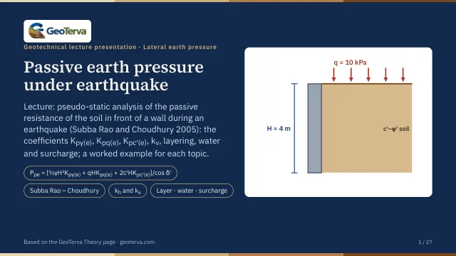 PDF
Lecture slides
Ready-made slides for lectures and self-study
The mechanism, the derivation, the equations and the figures of this page, in teaching order. Every slide links back to its chapter.
1The pseudo-static passive forceSubba Rao & Choudhury (2005).
During an earthquake the passive resistance in front of a wall drops: the inertia of the soil wedge helps to push it out. Subba Rao & Choudhury (2005) extended the curved-surface limit-equilibrium analysis of passive pressure (a log spiral with a planar part) with pseudo-static forces kₕW and kᵥW, for a vertical wall, a level c′–φ′ backfill with a surcharge q, wall friction δ′ and wall adhesion c′ₐ. The passive force is
The three coefficients are the components normal to the wall — hence the division by cos δ′. The γ part acts at H/3, the q and c′ parts at H/2:
2The coefficientsThe charts and the table of the coefficients.
Subba Rao & Choudhury (2005) give Kpγ(e) and Kpq(e) as charts for φ′ = 10°, 20°, 30°, 40°, δ′/φ′ = 0.5 and 1, and kᵥ = 0 or kᵥ = kₕ. The module carries the curves of these charts, resampled at Δkₕ = 0.01, and interpolates between them: linearly in kₕ and δ′/φ′, log-linearly in φ′. It does not extrapolate: φ′ must lie in 10–40° and δ′ in φ′/2 to φ′.
The coefficients fall as kₕ grows, and much faster when the vertical acceleration acts too (kᵥ = kₕ). Each curve ends where the passive resistance is exhausted; the module stops beyond it. At kₕ = 0 the charts are static passive coefficients: for φ′ = δ′ = 40°, Kpγ(e) = 14.49, against Kₚ cos δ′ = 14.45 from the log-spiral module. The module takes any 0 ≤ kᵥ ≤ kₕ given by the user (upward, the sense unfavourable to a passive force; kᵥ = 0.5kₕ is a usual choice) and interpolates linearly between the curves of kᵥ = 0 and kᵥ = kₕ at the same kₕ; checked with the pseudo-static Coulomb coefficient, whose exact kᵥ dependence is known, this errs by less than 0.4 %, on the low side.
Kpc′(e) is tabulated for φ′ = 10–40°, δ′/φ′ = 0.5 and 1, and c′ₐ = 0 or c′ₐ/c′ = tan δ′/tan φ′; for φ′ = 40° and δ′/φ′ = 1 it is 5.95 with c′ₐ = 0 and 5.97 with adhesion.
3Layers, water and surchargeA layered soil with a water table (this module).
The charts are drawn for one soil behind a vertical wall with a level surface, so the geometry stays so. The module takes the soil in layers with level boundaries: each layer takes its own coefficients, the overburden of the layers above it (and the surcharge q) acting on it as a surcharge through Kpq(e), its own weight through Kpγ(e) and its cohesion through Kpc′(e). Normal to the wall, per unit depth,
and along the wall σn tan δ′ of the layer; for one soil this is Eq. (1). A level water table gives γ′ = γsat − γw below it, and u acts normal to the wall. In the earthquake the pore water either moves with the soil (restrained) or, in a highly permeable soil, does not (free); the inertia is then that of the saturated or of the dry mass on the buoyant weight, and the charts are read at a larger seismic coefficient below the water table:
Free pore water adds its hydrodynamic pressure (Westergaard 1933), 7/8 khγw√(dwz′), which the module takes off the resistance — the phase unfavourable to a passive force. A vertical coefficient keeps its value below the water table: the charts are interpolated there at kv/kh,w. This layered form is the module’s engineering extension, not a solution of the literature; beyond the end of a chart curve (where the passive resistance runs out) the module stops.
4Worked exampleThe wall the module opens with.
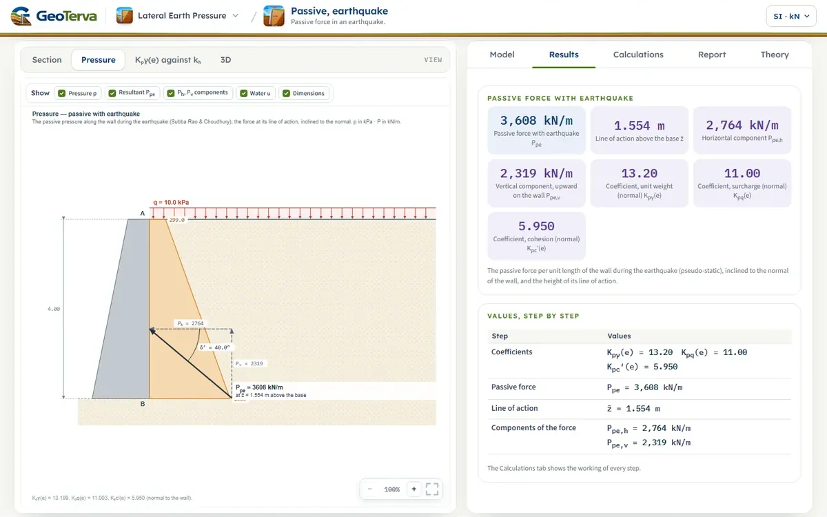
A vertical wall H = 4 m with φ′ = δ′ = 40°, γ = 17.5 kN/m³, q = 10 kN/m², c′ = 10 kN/m², c′ₐ = 0, kᵥ = 0 and kₕ = 0.3. From the charts (δ′/φ′ = 1):
The module opens with this example.
5ReferencesSources.
- Das, B.M. (2018). Principles of Geotechnical Engineering, 9th ed. Cengage Learning.
- Subba Rao, K.S. and Choudhury, D. (2005). Seismic passive earth pressures in soils. Journal of Geotechnical and Geoenvironmental Engineering, ASCE, 131(1), 131–135.
- Westergaard, H.M. (1933). Water pressures on dams during earthquakes. Transactions ASCE, 98, 418–433.
From theory to your own design
Find the seismic passive force on your own wall in minutes
- The passive force during the earthquake, its components and its line of action, step by step
- The seismic coefficients of the pseudo-static analysis for your wall and your soil
- A layered soil, a water table and a surcharge
- A clean calculation report, saved as a PDF. Works on your phone and in your browser