
On this page · 6 chapters
The horizontal pressure that a triangular surface load, parallel to a vertical wall, adds to the wall: the radii and angles at a depth, the pressure as the superposition of line loads, the resultant and its line of action. The figure and every number are computed from the module's own equations.
 PDF
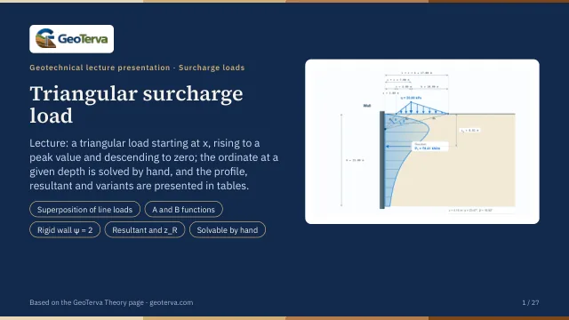
Lecture slides
Ready-made slides for lectures and self-study
The mechanism, the derivation, the equations and the figures of this page, in teaching order. Every slide links back to its chapter.
1Triangular load on a wallWhat the module computes.
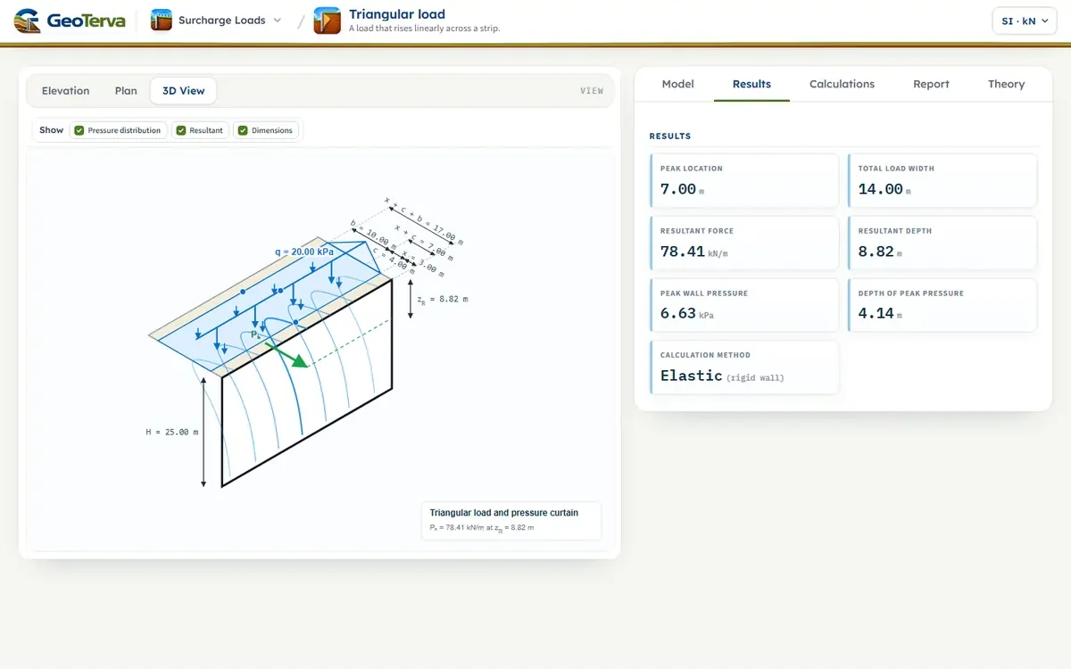
The surface surcharge begins at a horizontal distance x from the wall. Its intensity increases linearly from zero to the peak value q over a width c, then decreases linearly back to zero over a width b. At each wall depth z the geometry is described by the three radii R₁, R₂ and R₃ and the two angles α and β.
Variables
- — total wall height
- — distance from the wall to the start of the load
- — width of the increasing branch
- — width of the decreasing branch
- — peak surcharge intensity
- — depth below ground level
2Radii and anglesThe geometry at a depth z.
At the depth z the three rays from the wall point to the start of the load, to its peak and to its end have the lengths
and the two angles between them are
Use radians in the pressure equation. Degree values are useful only for reporting.
3Horizontal pressureThe superposition of line loads.
A triangular load is a continuous row of line loads, each of intensity w(s)·ds. Adding their elastic horizontal stresses (Flamant) over the load gives the pressure exactly:
With s₁ = x, s₂ = x + c, s₃ = x + c + b, R² = s² + z² and the two functions
the integral gives
A₂ − A₁ and A₃ − A₂ contain the angles α and β; B₂ − B₁ and B₃ − B₂ contain ln(R₂/R₁) and ln(R₃/R₂). The same superposition applied to a uniform strip gives the familiar (q/π)[β − sin β·cos 2α] exactly, which is how this expression is checked. ψ = 1 is the half-space (no wall); ψ = 2 is a rigid wall that does not yield, which doubles the horizontal stress — the module's default, as for the other surcharge loads. Repeating the calculation through the wall height gives σH(z); the pressure is zero at the ground surface.
| z (m) | R1 (m) | R2 (m) | R3 (m) | α (°) | β (°) | σH half-space (kPa) | σH rigid wall (kPa) |
|---|---|---|---|---|---|---|---|
| 1.00 | 3.16 | 7.07 | 17.03 | 10.305 | 4.764 | 1.48 | 2.97 |
| 2.50 | 3.91 | 7.43 | 17.18 | 20.152 | 11.288 | 2.91 | 5.81 |
| 5.00 | 5.83 | 8.60 | 17.72 | 23.499 | 19.148 | 3.25 | 6.49 |
| 7.50 | 8.08 | 10.26 | 18.58 | 21.224 | 23.169 | 2.64 | 5.29 |
| 10.00 | 10.44 | 12.21 | 19.72 | 18.293 | 24.542 | 1.98 | 3.95 |
| 15.00 | 15.30 | 16.55 | 22.67 | 13.707 | 23.559 | 1.07 | 2.14 |
| 20.00 | 20.22 | 21.19 | 26.25 | 10.759 | 21.074 | 0.6020 | 1.20 |
| 25.00 | 25.18 | 25.96 | 30.23 | 8.799 | 18.573 | 0.3615 | 0.7230 |
4Resultant and line of actionArea of the diagram and its first moment.
The resultant surcharge force per unit length of wall and its depth below the ground are the area of the diagram and its first moment:
The module integrates both numerically to full precision. For the example, PH = 78.41 kN/m (rigid wall) or 39.21 kN/m (half-space), at zR = 8.82 m below ground level in both.
5Worked exampleThe sequence by hand and one ordinate.
The data are H = 25.00 m, x = 3.00 m, c = 4.00 m, b = 10.00 m and q = 20.00 kPa; the example is fixed and does not follow the inputs of the interface. By hand, the sequence is:
- Define H, x, c, b and q — they define the whole triangular load — and choose ψ.
- Select a depth z and evaluate the ordinate required along the wall.
- Calculate R₁, R₂, R₃ (Eq. (1)–Eq. (3)) from x, x + c and x + c + b.
- Calculate α and β (Eq. (4), Eq. (5)), the angular differences between the three rays.
- Calculate σH from Eq. (8): evaluate A and B at s₁, s₂, s₃ and substitute, with the angles in radians.
- Repeat and integrate to build the pressure profile, then PH and zR.
The ordinate at z = 5.00 m
Results at the default inputs
PH = 78.41 kN/m (rigid wall) and 39.21 kN/m (half-space), with zR = 8.82 m below ground level.
6ReferencesSources.
- Das, B.M. (2016). Principles of Foundation Engineering, 8th ed. Cengage Learning; this page follows it.
From theory to your own design
Find the pressure from your own triangular load in minutes
- The pressure with depth, and the resultant with its height
- A load rising linearly from zero across a strip
- Elevation, plan and 3D views
- A clean calculation report, saved as a PDF. Online: nothing to install, no dongle, on a phone, a tablet or a PC