
On this page · 8 chapters
The horizontal pressure that a concentrated load on the ground adds to a vertical wall: the elastic solution for a rigid wall and the Terzaghi–NAVFAC chart, the pressure at a depth, the resultant and its location, the distribution along the wall and several loads on one line. The figures and every number are computed from the module's own equations.
 PDF
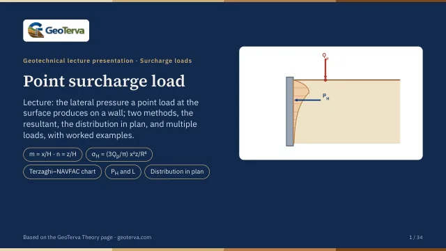
Lecture slides
Ready-made slides for lectures and self-study
The mechanism, the derivation, the equations and the figures of this page, in teaching order. Every slide links back to its chapter.
1Point load on a wallWhat the module computes.
A concentrated surface load Qp creates a three-dimensional stress field in the soil. When a vertical wall lies within that influence zone, part of the stress increase appears as an additional horizontal pressure on the wall. The module determines the pressure variation with depth on the load's own perpendicular to the wall, its resultant and line of action, and the distribution of the pressure along the wall in plan.
Let H be the wall height, x the horizontal distance from the wall to the point load, z the depth below the ground surface and y the distance along the wall from the load's perpendicular. Two dimensionless ratios are used:
Variables
- — concentrated point load acting at the ground surface
- — total wall height used in the surcharge formulation
- — horizontal distance from the wall to Qp
- — elastic method: the least distance a load is calculated at (0.30 m)
- — distance along the wall from the load's perpendicular
- — depth below the ground surface at which the pressure is evaluated
- — distance from the load to the point on the wall, √(x² + y² + z²)
- — lateral surcharge pressure on the load centreline at the depth z
- — lateral surcharge pressure away from the centreline, in plan
- — resultant horizontal surcharge force per unit length of wall at the load's section (y = 0), the area of the elevation diagram
- — distance from the wall base to the line of action of the resultant (the centroid of the diagram)
- — dimensionless area of the diagram and its moment about the base
- — index of a point load when there are several (1, 2, 3)
- — chart method: plan angle measured away from the load centreline
2The two methodsElastic for a rigid wall, and the chart.
Two established formulations are offered. Both describe a wall that does not yield; they differ most for a load close to the wall.
Elastic · rigid wall (the default)
Terzaghi – NAVFAC chart
Two cases, by the distance ratio: Case 1 for m ≤ 0.4 and Case 2 for m > 0.4 (their equations are in chapter 4); the centreline pressure is reduced along the wall by σ′H = σH cos²(1.1θ). The distance has an effect only beyond 0.4H; a load inside 0.4H is taken at 0.4H.
The elastic method is the stress a surface point load produces in an elastic half-space (Boussinesq), doubled for a smooth unyielding wall: a mirror-image load on the far side of the wall face cancels the lateral movement there and doubles the horizontal stress exactly (Mindlin 1936). Pressures measured on relatively rigid (though not smooth) retaining walls under a truck-wheel load were of the same order — roughly double the half-space values, with some points above double, partly put down to shear on the rough wall face — and the same factor of 2 is the rigid-wall factor applied to the Boussinesq solution in practice. Poisson's ratio is taken as 0.5, for which the formula is exact; on the load's own perpendicular (y = 0) a smaller ratio lowers the pressure and predicts tension near the top of the wall.
The chart method is the one of Terzaghi (1954), long used in design practice. It also assumes an unyielding wall, but Terzaghi stopped the distance effect at m = 0.4: a load closer than 0.4H is drawn as if it stood at 0.4H, so moving it within that range changes nothing. Because the method rests on elastic theory and tests on rigid unyielding walls, it is conservative for sheet pile walls, which deflect; heavy equipment within a few feet of the wall is usually considered separately.
For a load within 0.4H the two part company: the chart keeps one diagram, while the elastic solution concentrates a growing pressure near the top of the wall. Farther out they give resultants of the same order, the elastic one acting somewhat higher. With H = 15 m and Qp = 38 kN:
| x (m) | m | Elastic · rigid wall | Terzaghi – NAVFAC chart | |||
|---|---|---|---|---|---|---|
| PH (kN/m) | L (m) | PH (kN/m) | L (m) | Case | ||
| 0.30 | 0.020 | 40.32 | 14.70 | 1.99 | 8.81 | Case 1 |
| 1.00 | 0.067 | 12.09 | 14.01 | 1.99 | 8.81 | Case 1 |
| 2.00 | 0.133 | 6.03 | 13.05 | 1.99 | 8.81 | Case 1 |
| 3.00 | 0.200 | 4.00 | 12.15 | 1.99 | 8.81 | Case 1 |
| 4.00 | 0.267 | 2.97 | 11.33 | 1.99 | 8.81 | Case 1 |
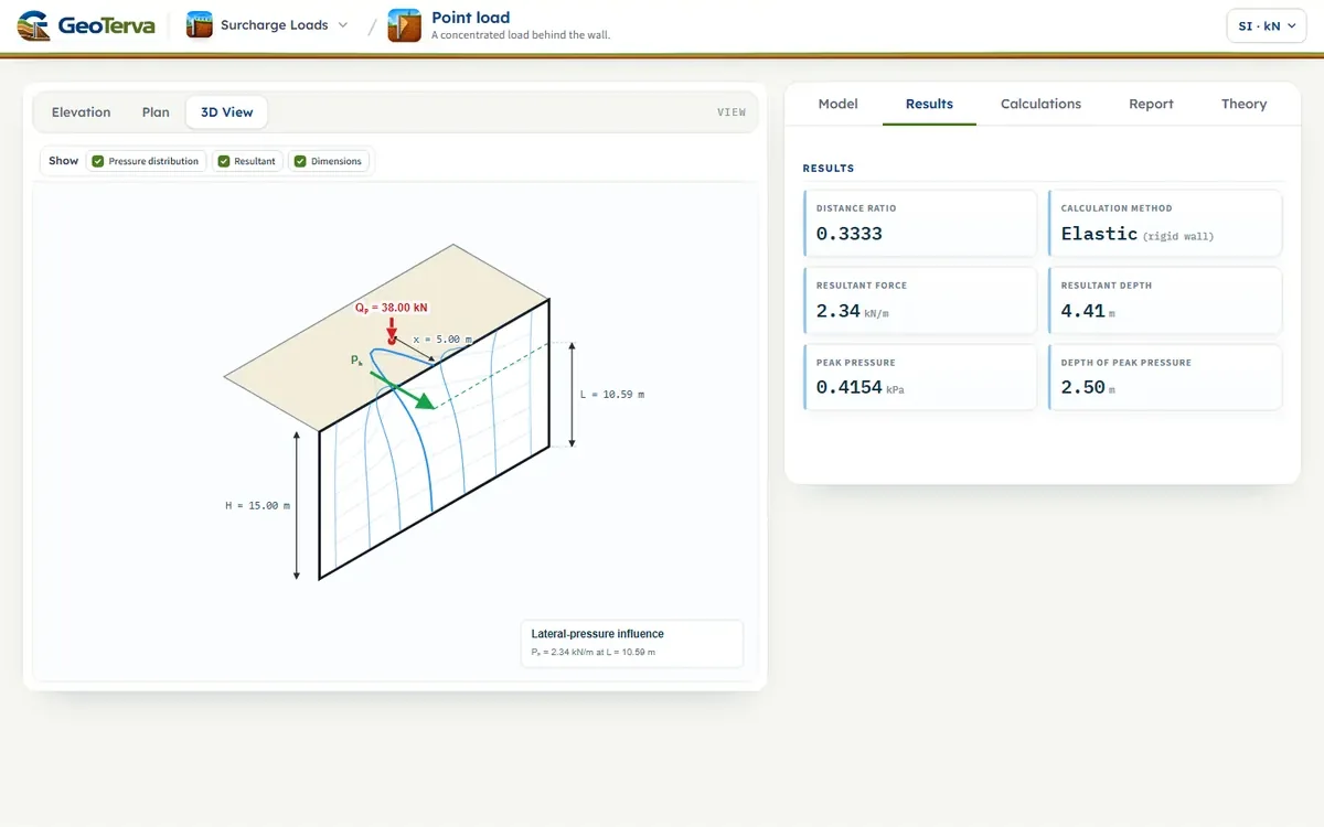
| 5.00 | 0.333 | 2.34 | 10.59 | 1.99 | 8.81 | Case 1 |
| 6.00 | 0.400 | 1.91 | 9.94 | 1.99 | 8.81 | Case 1 |
| 8.00 | 0.533 | 1.35 | 8.87 | 1.38 | 7.61 | Case 2 |
| 10.00 | 0.667 | 1.00 | 8.05 | 0.9755 | 6.74 | Case 2 |
| 15.00 | 1.000 | 0.5213 | 6.80 | 0.4402 | 5.45 | Case 2 |
3Elastic methodPressure, peak and closed-form resultant.
On the load's own perpendicular (y = 0), with m and n:
The diagram peaks at z = x/2, where σH,max = 0.2733 Qp/x² (for a load beyond 2H the peak is at the base). Its area and its moment about the base have closed forms, so the resultant and its height above the base are exact:
with PH = (Qp/H)·I₀ and L = H·I₁/I₀ (chapter 5). As the load approaches the wall the solution becomes singular: PH grows as Qp/(πx) and the peak, 0.2733 Qp/x², grows without limit. No real load acts like that, because a load that close is spread over a footprint, which may bear partly on the wall or its capping. The module therefore calculates a load nearer than xmin = 0.30 m (about 1 ft; a practical cut-off chosen for this module, not a limit that comes from the theory) at xmin, and flags it; a load that close should be considered separately, for example as an area load or a direct load on the wall.
Beyond xmin the distance still counts, but the elastic equations become unreliable for a load within a critical distance of about 0.4H — the same range in which the chart stops the distance effect (x < 6.00 m in the example). Elastic results for a load between xmin and 0.4H therefore call for engineering judgement, and the chart method gives a comparison.
4Chart methodCase 1 and Case 2 of Terzaghi–NAVFAC.
At each depth calculate n = z/H, then select the equation by m:
The Case 1 equation contains no m: it is the Case 2 equation evaluated at m = 0.4 (1.77 × 0.16 = 0.2832, printed as 0.28), so a load within 0.4H — 6.00 m in the example — gives the same diagram, PH and L wherever it stands. Because of the rounding, PH steps up by 1.1 % as the load crosses 0.4H; L is continuous there. The Elevation view marks 0.4H on the ground line when this method is chosen, as in the figure below.
5Resultant and its locationPH, L and the integrals I₀, I₁.
For either method the resultant PH is the area of the pressure diagram over the wall height, and L is the height of its centroid, measured upward from the base of the wall; the resultant therefore acts at the depth H − L below the ground surface. PH is a force per unit length of wall at the load's own section (y = 0), where it is largest. A point load's pressure falls away along the wall (next chapter), so PH must not be multiplied by a length of wall to get a total force.
Writing σH = (Qp/H²)·f(n), the load and the height come outside the integrals, leaving two pure numbers of the diagram shape:
The elastic method evaluates them in closed form (Eq. (4)); the chart method numerically. The chart constants of chapter 4 are this same integral read at one value of m: at m = 0.4 it gives PH = 0.787 Qp/H and L = 0.587 H, at m = 0.6 it gives 0.457 Qp/H and 0.476 H; integrating rather than using one constant for every m > 0.4 keeps PH and L consistent with the drawn diagram as the load moves.
6Pressure in plan and several loadsAlong the wall; up to three loads on one line.
Elastic method
The formula of Eq. (2) already holds at any point of the wall: with R² = x² + y² + z², at a fixed depth the pressure falls along the wall as (R₀/R)⁵, R₀ being R at y = 0, and at a distance y its peak lies at z = √(x² + y²)/2.
Chart method
The centreline pressure is reduced according to the plan angle θ, measured at the load between the perpendicular to the wall and the line to the point on the wall in question:
θ = 0° is the load centreline, where σ′H = σH. The module holds the reduction at zero past the angle where 1.1θ reaches 90° (θ ≈ 81.8°), since the cosine-squared term would otherwise start rising again beyond that point.
Several point loads on one line
Up to three loads can be entered, each with its own distance xi and magnitude Qp,i. They stand on one line perpendicular to the wall, so every one of them is opposite the same wall section. The pressures are stress increments, so they add; each load keeps its own ratio mi = xi/H (and, with the chart, its own case):
The combined resultant acts where the moments about the base balance, which is also the centroid of the summed diagram. Along the wall in plan, each load's pressure is taken at that position (its own Ri, or its own θi with the chart) and the pressures add. Loads standing beside that line, at different positions along the wall, are not part of this model.
7Worked exampleThe sequence by hand and the default inputs.
Elastic method, at the module's default inputs: H = 15.00 m, x = 5.00 m and Qp = 38.0 kN. The example is fixed and does not follow the edits made in the interface. By hand, the sequence is:
- Read the basic data: define H, the method, and x and Qp for each load.
- Calculate m = x/H for each load (Eq. (1)). Elastic: a load nearer than xmin is taken at xmin. Chart: decide whether m ≤ 0.4 or m > 0.4.
- Calculate σH at the depths required (n = z/H) with the equation of the method, Eq. (3) or Eq. (5) and Eq. (6) for each load; add the loads.
- Calculate PH and L: PH = (Qp/H)·I₀ and L = H·I₁/I₀ for each load (Eq. (7)) — closed form for the elastic method, integrated for the chart; add the PH and balance the moments for L.
- Distribute along the wall: elastic — evaluate the formula at the offset y; chart — σ′H = σH cos²(1.1θ) (Eq. (9)).
Distance ratio
Peak pressure
Resultant and its location
Moving along the wall
The chart method applies its own reduction to its own centreline pressure at this depth, 0.1984 kPa:
Its pressure falls off more slowly along the wall (0.42 against 0.23 of the centreline value), but from a lower start.
8ReferencesSources.
- Das, B.M. (2016). Principles of Foundation Engineering, 8th ed. Cengage Learning; this page follows it.
- Terzaghi, K. (1954). Anchored bulkheads. Transactions of the ASCE, 119, 1243–1280.
- NAVFAC DM-7.02 (1986). Foundations and Earth Structures. Naval Facilities Engineering Command.
- Boussinesq, J. (1883). Application des Potentiels à l’Étude de l’Équilibre et du Mouvement des Solides Élastiques. Gauthier-Villars, Paris.
- Mindlin, R.D. (1936). Discussion: Pressure distribution on retaining walls. Proc. 1st Int. Conf. on Soil Mechanics and Foundation Engineering, Harvard, Vol. III, 155–156.
- Spangler, M.G. and Mickle, J.L. (1956). Lateral pressures on retaining walls due to backfill surface loads. Highway Research Board Bulletin 141.
- Bowles, J.E. (1996). Foundation Analysis and Design, 5th ed.
- Frazee, G. (2021). New formulations of Boussinesq solution for vertical and lateral stresses in soil. ASCE Practice Periodical on Structural Design and Construction, 26(2).
- USS Steel Sheet Piling Design Manual (1984); California Department of Transportation, Trenching and Shoring Manual — the chart method.
From theory to your own design
Find the pressure from your own point loads in minutes
- The pressure with depth and the resultant with its height
- Up to three point loads on one line, with the spread along the wall in plan
- Elevation, plan and 3D views
- A clean calculation report, saved as a PDF. Online: nothing to install, no dongle, on a phone, a tablet or a PC