
On this page · 5 chapters
The horizontal pressure that a long line load on the ground, parallel to a vertical wall, adds to the wall: the elastic solution for a rigid wall and the Terzaghi–NAVFAC chart, the pressure at a depth, the resultant and its line of action. The figure and every number are computed from the module's own equations.
 PDF
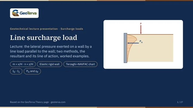
Lecture slides
Ready-made slides for lectures and self-study
The mechanism, the derivation, the equations and the figures of this page, in teaching order. Every slide links back to its chapter.
1Line load on a wallWhat the module computes.
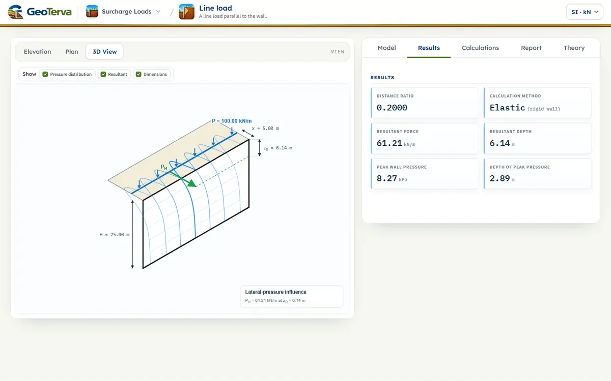
A surface line load P, a force per unit length, acts parallel to the wall at a horizontal distance x. The lateral surcharge pressure on the wall depends on the normalized load distance m = x/H and the normalized wall depth n = z/H.
Variables
- — surface line load per unit length, parallel to the wall
- — horizontal distance from the wall to the line load
- — wall height
- — depth below the ground surface
- — lateral surcharge pressure at the depth z
- — resultant force per unit length of wall
- — depth of the resultant below the ground surface
- — elastic method: the least distance a load is calculated at
2The two methodsElastic for a rigid wall, and the chart.
The two ratios of the geometry are
Elastic · rigid wall (the default of the module) — twice the horizontal stress that a line load produces in an elastic half-space (Flamant, Boussinesq), because an unyielding wall stops the soil at its face from moving; it holds for every distance:
A load nearer than xmin = 0.30 m is calculated at xmin, because the pressure peak, at n = m/√3, grows without limit as the line reaches the wall (the resultant itself stays finite).
Terzaghi – NAVFAC chart — the same equation for m > 0.4 and, for a line closer than 0.4H, the diagram held at m = 0.4:
The coefficient 0.203 is 4 × 0.16/π rounded, so the distance has no effect inside 0.4H. Use the same branch for the complete pressure profile: m is constant for a given model while n varies with the depth.
3Resultant and line of actionClosed forms and the two methods side by side.
For either method the resultant is the area of the diagram and its depth below the ground is where the first moment balances; with σH written as a function of n, the load and the height come outside the integrals:
Both integrals have closed forms. For the elastic equation, and for the chart when m > 0.4:
The chart resultant 0.64P/(m² + 1) is the first of these. For the chart with m ≤ 0.4:
where 0.5469 is the chart's 0.55P. With H = 25 m and P = 100 kN/m the two methods give:
| x (m) | m | Elastic · rigid wall | Terzaghi – NAVFAC chart | |||
|---|---|---|---|---|---|---|
| PH (kN/m) | zR (m) | PH (kN/m) | zR (m) | Case | ||
| 0.50 | 0.020 | 63.64 | 0.77 | 54.69 | 9.81 | Case 1 |
| 1.00 | 0.040 | 63.56 | 1.49 | 54.69 | 9.81 | Case 1 |
| 2.00 | 0.080 | 63.26 | 2.84 | 54.69 | 9.81 | Case 1 |
| 5.00 | 0.200 | 61.21 | 6.14 | 54.69 | 9.81 | Case 1 |
| 8.00 | 0.320 | 57.75 | 8.56 | 54.69 | 9.81 | Case 1 |
| 10.00 | 0.400 | 54.88 | 9.81 | 54.69 | 9.81 | Case 1 |
| 12.50 | 0.500 | 50.93 | 11.05 | 50.93 | 11.05 | Case 2 |
| 15.00 | 0.600 | 46.81 | 12.02 | 46.81 | 12.02 | Case 2 |
| 25.00 | 1.000 | 31.83 | 14.27 | 31.83 | 14.27 | Case 2 |
4Worked exampleThe sequence by hand and one ordinate.
The data are H = 25.00 m, x = 5.00 m and P = 100.00 kN/m; the example is fixed and does not follow the inputs of the interface. By hand, the sequence is:
- Enter H, x and P — the wall height, the offset and the intensity of the line load — and the method.
- Calculate m = x/H (Eq. (1)); with the chart it selects the governing equation.
- Select a depth z and calculate n = z/H.
- Calculate σH with Eq. (2) or, for the chart with m ≤ 0.4, Eq. (3).
- Resultant from the closed forms: PH = P·I₀ and zR = H·I₁/I₀ (Eq. (4), Eq. (5)).
The ordinate at z = 5.00 m
The resultant
5ReferencesSources.
- Das, B.M. (2016). Principles of Foundation Engineering, 8th ed. Cengage Learning; this page follows it.
- Terzaghi, K. (1954). Anchored bulkheads. Transactions of the ASCE, 119, 1243–1280.
- NAVFAC DM-7.02 (1986). Foundations and Earth Structures. Naval Facilities Engineering Command.
From theory to your own design
Find the pressure from your own line load in minutes
- The pressure with depth, and the resultant with its height
- The two branches of the solution for loads near and far from the wall
- Elevation, plan and 3D views
- A clean calculation report, saved as a PDF. Online: nothing to install, no dongle, on a phone, a tablet or a PC