
On this page · 5 chapters
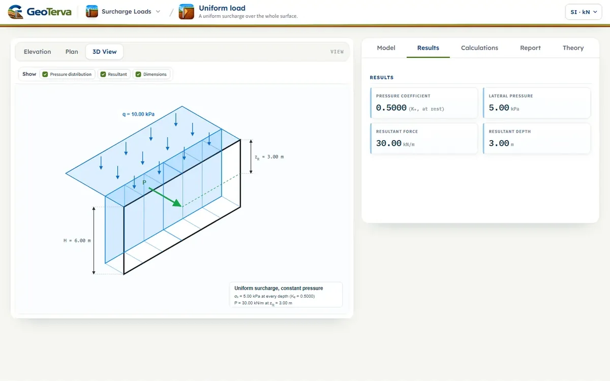
The horizontal pressure that a uniform load over the whole ground surface behind a wall adds to the wall: the coefficient K, the pressure, its resultant and line of action. The figure and every number are computed from the module's own equations.
 PDF
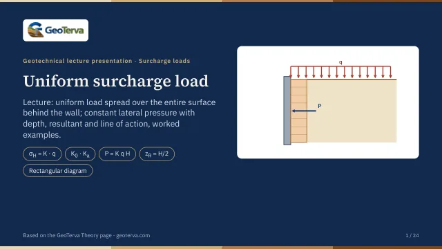
Lecture slides
Ready-made slides for lectures and self-study
The mechanism, the derivation, the equations and the figures of this page, in teaching order. Every slide links back to its chapter.
1Uniform load on a wallWhat the module computes.
A uniformly distributed load q spread over the whole ground surface behind the wall raises the vertical stress by q at every depth. The wall feels a fraction of it, set by the lateral earth-pressure coefficient K, so the added pressure is the same from the top of the wall to its base.
Variables
- — uniform surcharge over the retained surface
- — wall height
- — effective friction angle of the retained soil
- — lateral earth-pressure coefficient (K₀, Kₐ or entered)
- — added lateral pressure, constant with depth
- — resultant force per unit length of wall
- — depth of the resultant below the ground
2Lateral pressureK·q at every depth, and the choice of K.
The pressure added to the wall is the load times the coefficient, the same at every depth z:
The coefficient follows the behaviour of the wall. A wall that is propped or otherwise cannot move keeps the soil in its at-rest state, and the default is the coefficient of Jaky for a normally consolidated soil — the same stance as the rigid-wall default of the other surcharge modules:
A wall that yields enough to mobilise the active state takes the Rankine coefficient of a vertical wall with level ground:
A coefficient from another source (an overconsolidated K₀, a Coulomb Kₐ for a sloping or rough wall) can be entered directly.
| φ′ (°) | Ka | K0 |
|---|---|---|
| 0 | 1.0000 | 1.0000 |
| 20 | 0.4903 | 0.6580 |
| 25 | 0.4059 | 0.5774 |
| 30 | 0.3333 | 0.5000 |
| 35 | 0.2710 | 0.4264 |
| 40 | 0.2174 | 0.3572 |
3Resultant and line of actionA rectangle: P = KqH at mid-height.
The diagram is a rectangle, so the resultant per unit length of wall and its line of action follow at once:
4Worked exampleH = 6 m, q = 10 kPa, φ′ = 30°.
The data are H = 6.00 m, q = 10.00 kPa and φ′ = 30°; the example is fixed and does not follow the inputs of the interface.
Coefficient — from Eq. (2) and Eq. (3):
Pressure — from Eq. (1):
Resultant — from Eq. (4) and Eq. (5):
5ReferencesSources.
- Das, B.M. (2016). Principles of Foundation Engineering, 8th ed. Cengage Learning; this page follows it.
- Jaky, J. (1944). The coefficient of earth pressure at rest. Journal of the Society of Hungarian Architects and Engineers, 7, 355–358.
- Rankine, W.M.J. (1857). On the stability of loose earth. Philosophical Transactions of the Royal Society of London, 147, 9–27.
From theory to your own design
Find the pressure from your own surcharge in minutes
- The constant pressure and its resultant at mid-height
- The coefficient K chosen for your wall
- Elevation and plan views
- A clean calculation report, saved as a PDF. Online: nothing to install, no dongle, on a phone, a tablet or a PC