
On this page · 5 chapters
Rankine's active and passive earth pressure on a vertical frictionless wall with a level backfill: the plastic-equilibrium states, cohesionless and cohesive soils, surcharge, water and tension cracks. The figures are computed from the equations.
 PDF
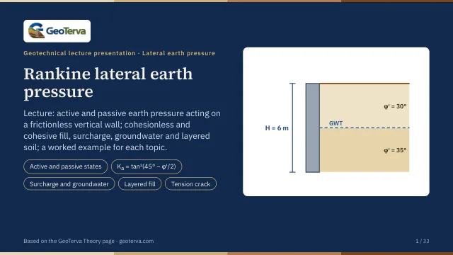
Lecture slides
Ready-made slides for lectures and self-study
The mechanism, the derivation, the equations and the figures of this page, in teaching order. Every slide links back to its chapter.
1Active and passive statesRankine's plastic equilibrium.
Rankine (1857) looked at a soil mass in plastic equilibrium — every point on the verge of failure. Behind a frictionless vertical wall that moves away from the soil the horizontal stress falls from its at-rest value K₀σ′ₒ until the Mohr circle touches the failure envelope: the active state. Pushed into the soil, the horizontal stress rises above σ′ₒ until the circle touches the envelope on the other side: the passive state.
From the geometry of the circle touching the envelope τf = c′ + σ′ tan φ′:
With the coefficients
the equations read σ′ₐ = Kₐσ′ₒ − 2c′√Kₐ and σ′ₚ = Kₚσ′ₒ + 2c′√Kₚ.
A wall of limited height reaches these states when it rotates about its base far enough (the at-rest module lists the typical movements needed): the soil in the triangular wedge behind it bounded by a slip plane is then in plastic equilibrium, and the pressure on the wall follows the equations above.
2Cohesionless backfillSurcharge, water, layers.
Cohesionless soil, level backfill. With c′ = 0 the pressures grow linearly with depth, and the forces per unit length of the wall act at H/3 above the base:
Surcharge and water. A uniform surcharge q adds qKₐ at every depth (a rectangle). Below the water table the effective stress uses γ′ = γsat − γw, and the water pressure u = γw(z − H₁) adds in full:
and Pₚ in the same way with Kₚ. In a layered backfill each layer takes its own K, so the diagram steps at every boundary where φ′ changes; σ′ₒ itself is continuous.
3Cohesive backfillTension zone and cracks.
In a c′–φ′ soil the active pressure is negative near the top. It becomes zero at
Soil cannot pull on the wall: with time tension cracks open down to z₀ and the soil loses contact there. The force is then the area of the positive part only:
Before cracking, the whole diagram counts, Pₐ =½KₐγH² − 2√Kₐ c′H — a smaller force; the module offers both, cracks being the usual design assumption. With a surcharge or several layers the zero point moves; the module finds it where the diagram crosses zero.
Passive case. Cohesion adds everywhere: σ′ₚ = 2c′√Kₚ at the top and
4Worked examplesSand and c′–φ′ soil, layers and a water table, active and passive.
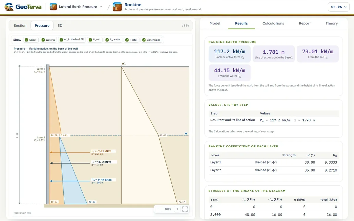
The table lists the force per unit length of the wall for six walls, as the module gives it; the module opens with case 3 (two sand layers, water table at 3 m), which is worked step by step below the table.
| No. | Case | Coefficient | Force |
|---|---|---|---|
| 1 | sand, H = 6 m, γ = 16 kN/m³, φ′ = 36°, active | Kₐ = 0.2596 | 74.77 |
| 2 | the same wall, passive | Kₚ = 3.852 | 1109.3 |
| 3 | two sands, H = 6 m: 3 m with γ = 16 kN/m³, φ′ = 30° over 3 m with γsat = 18 kN/m³, φ′ = 35°; water table at 3 m; active | Kₐ = 1/3, 0.271 | 117.15 (z̄ 1.78) |
| 4 | c′–φ′ soil, H = 4 m, γ = 15 kN/m³, φ′ = 26°, c′ = 8 kPa, q = 10 kPa; active, tension cracks | z₀ = 1.04 m | 25.65 |
| 5 | the same wall, passive | Kₚ = 2.561 | 512.2 |
| 6 | US units: 2 ft of clayey soil (γ = 110 pcf, φ′ = 20°, c′ = 300 psf) over 3 ft of sand (γ = 108 pcf, φ′ = 30°); active, tension cracks | whole top layer in tension | 5.575 (382.0 lb/ft) |
Case 3 step by step. Kₐ₁ = (1 − sin 30°)/(1 + sin 30°) = 1/3 for the upper sand and Kₐ₂ = 0.271 for the lower one. At 3 m, σ′ₒ = 48 kN/m², so σ′ₐ = 16 kN/m² just above the boundary and 13.0 kN/m² just below; at 6 m, σ′ₒ = 48 + 3(18 − 9.81) = 72.57 kN/m², σ′ₐ = 19.67 kN/m² and u = 29.43 kN/m²:
5ReferencesSources.
- Das, B.M. (2018). Principles of Geotechnical Engineering, 9th ed. Cengage Learning.
- Rankine, W.M.J. (1857). On the stability of loose earth. Philosophical Transactions of the Royal Society of London, 147, 9–27.
From theory to your own design
Find the Rankine pressure on your own wall in minutes
- The active or the passive pressure layer by layer, with the resultants and their heights, step by step
- A cohesive soil with its tension zone, a water table and a surcharge
- The pressure diagrams drawn to scale beside the wall
- A clean calculation report, saved as a PDF. Works on your phone and in your browser