
On this page · 5 chapters
The vertical stress below a flexible strip load that increases linearly across its width, from the line-load solution. The figures are computed from the equations.
 PDF
Lecture slides
Ready-made slides for lectures and self-study
The mechanism, the derivation, the equations and the figures of this page, in teaching order. Every slide links back to its chapter.
1Scope and assumptionsA triangular strip load.
The slope of an embankment, a stockpile against a wall, the toe of a fill: a strip load whose intensity grows from nothing at one edge to q at the other. This module gives the vertical stress increase below such a linearly increasing strip of width B and infinite length; together with the uniform strip it builds the embankment load.
- Flexible strip; the load is q·x/B at 0 ≤ x ≤ B and zero elsewhere.
- The soil is a homogeneous, isotropic, linearly elastic half-space; plane strain.
- Δσz is an increase caused by the load only.
2DerivationIntegrating a line load of intensity (q/B) r dr.
The elemental strip at r carries (q/B) r dr per unit length. Treated as a line load at the horizontal distance x − r from A, and summed over the width:
The integral is elementary; written with the angles of the figure it becomes
with α in radians, and
δ is the angle from the vertical through A to the line to the high edge. Its sign matters: it is negative when the high edge lies on the +x side of A, as in the figure. With the arctangents of the equation the sign comes out by itself, and the result holds for every x — beside, under or beyond the strip.
3Chart and tableΔσz/q against 2x/B and 2z/B.
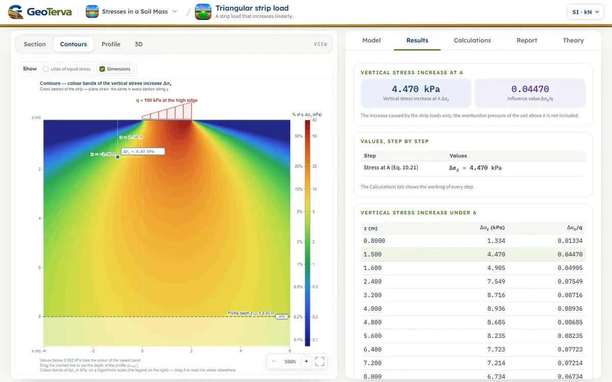
Near the surface the stress follows the load itself; deeper it spreads and its peak moves from the high edge toward the centroid of the load, two thirds of the width from the zero edge.
| 2x/B | 2z/B = 0.5 | 2z/B = 1 | 2z/B = 1.5 | 2z/B = 2 | 2z/B = 3 | 2z/B = 4 |
|---|---|---|---|---|---|---|
| -2 | 0.0008 | 0.0053 | 0.0140 | 0.0249 | 0.0448 | 0.0567 |
| -1 | 0.0041 | 0.0217 | 0.0447 | 0.0643 | 0.0854 | 0.0894 |
| 0 | 0.0749 | 0.1273 | 0.1528 | 0.1592 | 0.1469 | 0.1273 |
| 1 | 0.4797 | 0.4092 | 0.3341 | 0.2749 | 0.1979 | 0.1529 |
| 2 | 0.4220 | 0.3524 | 0.2952 | 0.2500 | 0.1872 | 0.1476 |
| 3 | 0.0152 | 0.0622 | 0.1010 | 0.1206 | 0.1259 | 0.1154 |
| 4 | 0.0019 | 0.0119 | 0.0285 | 0.0457 | 0.0691 | 0.0775 |
4Worked exampleEvery number computed by the module’s own code.
Measured from the surface, the angles are α₁ = tan⁻¹(1.5/3) = 26.57° to the high edge and α₂ = tan⁻¹(1.5/1) = 56.31° to the zero edge, so
the same as the equation gives: tan⁻¹[(−1 − 2)/1.5] = −63.43°. Then
The table above (2x/B = −1, 2z/B = 1.5) gives the same 0.0447. The module opens with this example. A strip may also be zero at its right edge: it is the mirror image of the strip of this example, and the same equation is used with x measured from the zero edge toward the high edge. Further strips, each with its own q, width, left edge and direction, are put in one by one with Add strip load (up to eight); the strips may not overlap — two may meet at an edge — and, the soil being elastic, the stresses add.
5ReferencesSources.
- Das, B.M. (2018). Principles of Geotechnical Engineering, 9th ed. Cengage Learning.
From theory to your own design
Find the stress below your own triangular load in minutes
- The vertical stress increase at a point below strips that rise linearly, either way round
- Contours of equal stress and a depth profile
- One strip or several
- A clean calculation report, saved as a PDF. Online: nothing to install, no dongle, on a phone, a tablet or a PC