
On this page · 15 chapters
Piles in a group do not carry, settle or move the way a single pile does. This page explains, section by section, how the module takes a group of piles under a rigid cap in layered ground: the load on every pile, the resistance of one pile alone, the efficiency of the group and its block failure, layer by layer, the elastic and the consolidation settlement, and the lateral load shared between the rows by p-multipliers; then a worked example whose every number is computed by the module’s own code, and the assumptions.
 PDF
Lecture slides
Ready-made slides for lectures and self-study
The mechanism, the derivation, the equations and the figures of this page, in teaching order. Every slide links back to its chapter.
1A group of pileswhat changes when piles stand together, and what the module gives
A single pile is analysed alone: its resistance, how far it settles, how far it moves sideways. A pile in a group is not alone. Piles are set in rows under a cap — a thick block of concrete that ties their heads together and takes the load of a column, a pier or a wall — and when they stand close the ground between and around them is asked to serve all of them at once. Three things follow, and the module takes each as a check of its own:
- The capacity. The soil between the piles is stressed by the shaft of every pile around it, so each pile carries less than it would alone: the group has an efficiency below one. With the piles close and the soil weak, the piles and the soil between them can also move down as one block, a deep footing of the size of the group, which is a limit of its own (Sections 4 to 7).
- The settlement. The load of a group spreads into the ground over the area of the whole group, not of one pile, and reaches the clay layers far below the tips. A group settles a good deal more than a single pile under the same load on each pile (Sections 8 and 9).
- The lateral response. A pile in the second row, or in the rows behind it, works in soil that the piles in front have already pushed and stressed. The front row takes more of a lateral load and the others less, and the group as a whole moves more than a single pile would under the load each of its piles carries (Sections 10 and 11).
The module takes a group of nx rows of ny piles under a rigid cap — a rectangular grid, or the piles at the corners of equilateral triangles — in up to eight layers of sand and clay with a water table. It gives the load on every pile (Section 2), the resistance of one pile alone, worked out from the ground and the installation (Section 3), the capacity of the group (Sections 4 to 7), the elastic and the consolidation settlement (Sections 8 and 9) and, when a lateral load is entered, the deflection of the cap and the load each row takes (Sections 10 and 11).
Layered ground: everything layer by layer
Most of the published methods were written for one soil — a group in clay, a group in sand. The ground under a real group is seldom one soil, and the module does not average it. Every layer gives the pile its own shaft resistance, the group its own efficiency, the block its own shear, the settlement its own consolidation and the lateral response its own p–y curve with its own p-multiplier. Section 6 shows how the layers enter the capacity, and Sections 9 and 10 the settlement and the lateral load.
2The load on every pilethe rigid cap, and the loads the piles are given
The cap is taken as rigid and the piles as identical vertical springs. A rigid cap moves as a plane — its settlement and its rotations are the only unknowns — so the shortening of a pile, and with it the load the pile takes, is a linear function of its position. This is the rule for a group of bolts. Every pile takes an equal share of the vertical load V and a part of each moment in proportion to its distance from the centroid of the group:
The piles of a rectangular grid stand symmetrically about the axes, so Σxy is zero, B = My/Σx² and C = Mx/Σy², and the sums are closed forms of the numbers of piles and their spacings:
The triangular arrangement
The piles may stand at the corners of equilateral triangles of side s instead: the piles of a row are s apart, the rows lie s√3/2 apart in the direction of the lateral load, and every second row is shifted along the row by s/2, so that every pile has six neighbours at the distance s. Such a group is denser than the grid of the same spacing, which holds one pile in s² of the plan where the triangular arrangement holds one in s²√3/2. The piles of a staggered group are no longer symmetric about both axes — with an even number of rows Σxy is not zero, and a moment about one axis loads the piles about the other — so the module takes the sums Σx², Σy² and Σxy from the positions of the piles themselves, and the two equations above are solved together. The group is centred on its centroid, the cap is the rectangle that encloses the piles, and the block of Section 7 is that rectangle.
My is positive when it adds compression to the piles on the +x side — the side a lateral load pushes towards — and Mx when it adds compression to the +y side. Both are taken at the base of the cap: a lateral load H at a height h above the base of the cap gives My = H h, and the module asks for the moments already taken to that level.
For the worked group — 3 rows of 3 piles at 1.80 m, V = 1600 kN, My = 900 kN·m — V/n is 177.8 kN, Σx² = 19.44 m² and B = 46.30 kN/m, so the rows, from the front, carry row 1: 261.1 kN, row 2: 177.8 kN, row 3: 94.4 kN. The largest load is on the front piles and the smallest on the back ones; none is in tension.
A pile in tension
Where the moment is large against the vertical load, the piles on the side away from the moment are unloaded and may be pulled up. The module lists such a pile as being in tension and works out what it can take. A pile resists tension by its shaft alone: each layer gives the shaft resistance of Section 3 by the method of its layer, a clay layer in full and a sand layer at three quarters of its resistance in compression (a reduction in common use for piles in sand), and the base gives nothing:
The largest tension on a pile is compared with Tu over the factor of safety, or with the allowable tension of one pile entered in the Design section, the lesser of the two governing. The piles in tension together are held by the lesser of two things: the piles themselves, each layer with the efficiency of its kind of soil (Sections 4 and 5), and the block of soil that encloses them, which is held down by its own weight — effective below the water table — and by the shear on its sides, with the same τ as the block in compression (Section 7):
The sum of the tensions on those piles is compared with Tg over the factor of safety. A single pile in tension has no block of its own and is held by Tind.
The most loaded pile
The check of the group compares the total load V with the capacity of the group, as if every pile took its share equally. With a moment on the cap the piles do not: the one on the side of the moment takes more than V/n, and a group can be within its own capacity while that pile is over its share. The module therefore compares the largest load on a pile with what one pile alone is allowed, its ultimate capacity over the factor of safety, and gives the statement beside Pmax in the Results:
The effect of the group is taken in the check of the group (Sections 4 to 7); the load of one pile is compared with the capacity of the pile alone and is not reduced by it. An allowable compression of one pile entered in the Design section is compared as well, and the lesser of the two governs.
What the rule assumes
- The piles are alike: the same section, length and head connection. A shorter or a stiffer pile would attract more of the load.
- The cap is rigid. A flexible cap would pass more of a column load to the piles directly under it.
- The piles resist the rotation of the cap by their own bending as well; the module takes the axial loads from the statics of the rigid cap, which is on the safe side for them, and gives the bending moments at the heads of the piles from the lateral analysis (Sections 10 and 11).
3The single pileone pile alone, layer by layer, and what the boxes fill themselves with
The capacity of a group is built on the capacity of one pile. The module therefore works out first the resistance of one pile of the group acting alone — layer by layer, from the ground and the installation — and applies the group effect to it (Section 4 onwards). No resistance of a single pile is entered: each layer of the shaft takes the method chosen for its own soil, and the base takes the method chosen for the soil it bears on. The methods are those of the source, as the module for a pile through layered ground applies them.
The effective stress
The effective vertical stress ties the layers together. It is measured from the ground surface, so the soil above the base of the cap is in it, and it accumulates through every layer above the depth in question, with the moist unit weight above the water table and the submerged unit weight below it:
The stress is continuous from layer to layer; the unit shaft resistance is not. At a boundary the rule itself changes, and f can step up or down by a wide margin (Figure 3). That is the signature of a layered profile, and the reason the shaft is worked layer by layer.
The shaft in a sand layer
The K–δ method takes the unit resistance as the horizontal effective stress — K times the vertical — times the friction of the pile–soil interface. The vertical stress is taken down to the critical depth L′ = 15 D below the head of the pile and held at its value there below it, so a sand layer deeper than L′ gives one unit resistance over its whole thickness, wherever the boundaries of the layers fall:
K varies with depth in the ground — near the passive value at the top of the pile, and possibly below the at-rest value deeper down — so the source recommends an average for each kind of pile, which follows the installation, and δ′ between 0.5 φ′ and 0.8 φ′. The module fills K in from the installation and the φ′ of each sand layer, and δ′ as 0.75 φ′; both can be typed over. From load tests, Mansur and Hunter (1970) report average values of K = 1.65 for H-piles, 1.26 for steel pipe piles and 1.5 for precast concrete piles.
| Installation | K | Range in the source |
|---|---|---|
| Bored | K0 = 1 − sin φ′ | K0 (bored or jetted) |
| Driven | 1.4 K0 | K0 to 1.4 K0 (low displacement), K0 to 1.8 K0 (high displacement) |
| Jacked | 1.4 K0 | as for a driven pile |
The method of Coyle and Castello (1981) pairs a K read from their chart against L/D and φ′ with δ′ = 0.8 φ′ and the mean effective stress of the layer. It has no critical depth: the averaging takes its place.
The correlation was written for one sand driven in place; taken layer by layer, with the mean stress of each layer, it is the module’s extension of it.
The shaft in a clay layer
The α method takes a fraction of the undrained strength of the layer, with α read from a correlation that falls as the clay gets stronger (Terzaghi, Peck and Mesri, 1996):
| cu/pa | α | cu/pa | α |
|---|---|---|---|
| 0.1 | 1.00 | 1.2 | 0.42 |
| 0.2 | 0.92 | 1.4 | 0.40 |
| 0.3 | 0.82 | 1.6 | 0.38 |
| 0.4 | 0.74 | 1.8 | 0.36 |
| 0.6 | 0.62 | 2.0 | 0.35 |
| 0.8 | 0.54 | 2.4 | 0.34 |
| 1.0 | 0.48 | 2.8 | 0.34 |
The λ method of Vijayvergiya and Focht (1972) applies one coefficient to the effective stress and the undrained strength together, with λ read against the embedded length of the pile:
| L (m) | λ | L (m) | λ |
|---|---|---|---|
| 0 | 0.500 | 35 | 0.132 |
| 5 | 0.336 | 40 | 0.127 |
| 10 | 0.245 | 50 | 0.118 |
| 15 | 0.200 | 60 | 0.113 |
| 20 | 0.173 | 70 | 0.110 |
| 25 | 0.150 | 80 | 0.110 |
| 30 | 0.136 | 90 | 0.110 |
λ was written as one average over the whole length of a pile in clay. Taken layer by layer — λ at the length of the pile, with the mean stress and the strength of the layer — it is the module’s extension of the method.
The β method (Burland, 1973, with the overconsolidation adjustment after Meyerhof) works from the effective stress alone, through the remoulded drained friction angle of the layer, with K taken at rest and raised by √OCR for an overconsolidated clay:
The unit resistance of an α layer is one number for the layer, flat with depth; that of a λ layer is flat as well, on the mean stress of its layer; that of a β layer follows σ′v and grows with depth inside the layer.
The base
The base belongs to one layer: the one the tip stands in (a tip exactly on a boundary bears on the layer beneath it). What lies above enters a sand base through the effective stress q′ at the tip, built from every layer above, and a clay base not at all.
In a sand there are three routes. Meyerhof (1976) reads N*q from the friction angle of the layer and limits the result by ql:
| φ′ | 20° | 25° | 30° | 35° | 40° | 45° |
|---|---|---|---|---|---|---|
| N*q | 12.4 | 26.0 | 56.7 | 143.0 | 346.0 | 930.0 |
Vesic (1977) takes the mean effective stress at the tip and a factor of the rigidity index of the sand, so the stiffness of the sand enters as well as its strength; Es is m pa, with m = 250 for a medium sand as the box opens:
Coyle and Castello read N*q from their own chart against L/D and φ′, with no limit; the box fills in from the chart at the φ′ of the tip layer and can be typed over:
| φ′ | K at L/D = 10 | K at L/D = 20 | K at L/D = 30 | N*q at L/D = 10 | N*q at L/D = 20 | N*q at L/D = 30 |
|---|---|---|---|---|---|---|
| 30° | 0.91 | 0.60 | 0.40 | 28.7 | 30.8 | 28.9 |
| 32° | 1.23 | 0.82 | 0.54 | 34.9 | 37.5 | 35.2 |
| 34° | 1.84 | 1.23 | 0.81 | 41.8 | 44.9 | 42.2 |
| 36° | 3.02 | 2.01 | 1.33 | 55.2 | 59.5 | 56.4 |
In a clay under undrained loading the friction angle is zero and the base resistance is a multiple of the undrained strength of the layer. Meyerhof takes the factor 9. Vesic builds it from the rigidity index of the clay, which in undrained loading reduces to a closed form in cu, with Irr = 347 cu/pa − 33 and at most 300; the correlation has a value from cu of about 10 kPa upwards, and for a softer clay the module asks for the factor 9:
A bored pile: the drilled-shaft rules
A bored pile is cast in a hole and displaces nothing: the clay at the wall of the hole softens as it takes up water, debris can collect under the base, and the base needs a larger settlement to develop its resistance. The source gives such a pile rules of its own, and the module applies each half where it belongs — the shaft rule over the clay layers that take α, and the base rule when the base stands in a clay. The adhesion factor is no longer the one of the driven pile (O’Neill and Reese, 1999):
and f is set to zero over two lengths of the shaft in an α layer: the top 1.5 m, the ground most disturbed by the work and the most likely to shrink away from the shaft, and the bottom diameter, over which the base is already mobilising the soil. The module applies both as a window on the integration, so the thicknesses of the layers, which also set depth and effective stress, are untouched; a sand layer keeps its K–δ or Coyle and Castello rule over its whole length in the pile, and the window belongs to the α procedure alone.
The base of a bored pile in a clay is worked from the clay beneath it, as the mean undrained strength cub over the 2 Db below the base (Reese and O’Neill, 1989), so the ground has to be described that far below the base; where the profile stops short, the deepest layer is taken to continue. A wide base would need an unacceptable settlement to reach qp, and for Db above 1.91 m the value is reduced by Fr:
Driven, bored and jacked
The installation decides which rules the pile follows. A jacked pile displaces the ground as a driven one does and follows the rules of a driven pile.
| Rule | Driven | Bored | Jacked |
|---|---|---|---|
| K in a sand layer (K–δ method) | 1.4 K0 | K0 | 1.4 K0 |
| α in a clay layer | the series of Table 2 | 0.55 up to cu/pa = 1.5, then down to 0.45 | as for a driven pile |
| Length of an α layer that carries friction | the whole length in the pile | not the top 1.5 m and not the bottom D | the whole length in the pile |
| Coyle and Castello (shaft, base) and λ | used | calibrated on driven piles; another method is asked for | used |
| Base in a clay | Meyerhof or Vesic | Meyerhof, Vesic or Reese and O’Neill | Meyerhof or Vesic |
| Efficiency of a sand layer (Section 5) | the chart of driven piles | AASHTO LRFD | the chart of driven piles |
What the boxes fill themselves with
- K of a sand layer: K0 of the layer for a bored pile, 1.4 K0 for a driven or a jacked one; δ′ is 0.75 φ′ of the layer.
- K of Coyle and Castello for a sand layer and their N*q at the base: read from their charts at the φ′ of the layer and the L/D of the pile.
- α of a clay layer: from cu of the layer and the installation (Table 2, or the drilled-shaft rule).
- φ′R = 30° and OCR = 1 of a β layer, and m = Es/pa = 250 of Vesic’s base in a sand: values of the ground, entered with it.
Each box can be typed over, and the value typed is the one the sheet uses.
The worked pile
For the worked group of Section 13 — a bored pile 0.60 m wide and 14 m long, with its head at the ground — the boxes of the Model tab open with the numbers below, and one pile alone gives:
| Layer | Soil | Method | Numbers of the boxes | f (kPa) | Q (kN) |
|---|---|---|---|---|---|
| Layer-1 | sand, φ′ = 32° | K–δ | K = 0.47, δ′ = 24° | 6.6 | 50 |
| Layer-2 | clay, cu = 50 kPa | α | α = 0.55, friction over 6.0 m of 6.0 m | 27.5 | 311 |
| Layer-3 | clay, cu = 90 kPa | α | α = 0.55, friction over 3.4 m of 4.0 m | 42.1 | 317 |
| Base | clay (Layer-3) | Meyerhof | N*c = 9, cu = 90 kPa | 810 | 229 |
| One pile alone | Qu = Qs + Qp | 907 |
4The efficiency of the grouphow close piles carry less, and the equations of the source
Far apart, each pile carries what it would carry alone. As the piles come together the zones of soil each of them shears and stresses begin to overlap, and each carries less. The efficiency of the group is the ratio of its capacity to the sum of the capacities of its piles alone:
The source gives three empirical equations for a group of n1 by n2 piles of width D at a centre-to-centre spacing d. The first is that of Converse and Labarre:
The second is the Los Angeles group-action equation, and the third that of Seiler and Keeney, in which d is taken in feet:
| s / D | Converse–Labarre | Los Angeles | Seiler–Keeney |
|---|---|---|---|
| 2.5 | 0.677 | 0.750 | 0.784 |
| 3.0 | 0.727 | 0.792 | 0.831 |
| 4.0 | 0.792 | 0.844 | 0.888 |
| 5.0 | 0.832 | 0.875 | 0.921 |
| 6.0 | 0.860 | 0.896 | 0.943 |
The triangular arrangement
The three equations were written for a rectangular group. Converse and Labarre’s counts the neighbouring pairs of piles — (nx − 1) ny pairs one behind the other and (ny − 1) nx side by side — each with the angle θ = tan⁻¹(D/d) of its own distance, and divides by 90 n. The module writes it the same way over the neighbouring pairs of a triangular arrangement: the nx (ny − 1) pairs of a row, at s, and the (nx − 1)(2 ny − 1) pairs of neighbouring rows, which make a zigzag, at s as well. For a rectangular grid it gives back the equation of the source exactly. For the triangular arrangement it is the module’s extension, not an equation of the source; it gives a lower efficiency than the grid of the same spacing, as every pile has more neighbours. The Los Angeles and Seiler–Keeney equations are written for the rectangular group, and the module gives them for it.
| s / D | rectangular grid | triangular arrangement |
|---|---|---|
| 2.5 | 0.677 | 0.569 |
| 3.0 | 0.727 | 0.636 |
| 4.0 | 0.792 | 0.723 |
| 5.0 | 0.832 | 0.777 |
| 6.0 | 0.860 | 0.813 |
The module uses the Converse–Labarre equation for a clay, and reduces by it the shaft resistance of every clay layer and the bearing of a pile whose base is in clay. In a sand it uses the rules of the next section. Which efficiency applies to which layer is the subject of Section 6. The equation takes the spacing of each direction (the pairs of a row at their spacing, the pairs of neighbouring rows at theirs; over the neighbouring pairs in the triangular arrangement). The sand rules, and the flag below, take the least distance between two piles: the smaller of the two spacings of a grid, the side s of the triangles of the other arrangement. A spacing of less than 2.5 diameters, the least the source gives for friction piles, is flagged: the group effect is large there, and the equations were written for wider spacings.
5Piles in sanddriven, jacked and bored: the chart of the source and AASHTO
In a sand the efficiency does not follow the equations of the last section. Driving a pile into loose or medium sand compacts the sand around it and between the piles, and a group of driven piles in such a sand carries as much as the sum of its piles alone — in the tests of Kishida and Meyerhof (1965), on a group of 3 by 3 piles, more. Only in a dense sand, with a friction angle above about 40°, where there is nothing left to compact, does a close spacing reduce the capacity: the curve of φ′ = 45° of those tests falls from 1.0 at a spacing of 7 diameters to 0.53 at 1 diameter.
For a driven pile in a sand layer (a jacked pile displaces the sand in the same way and takes the same) the module takes the chart of the source and never lets the efficiency rise above 1 — the gain from compaction is real but depends on how loose the sand was and in what order the piles were driven, so the module holds the efficiency at 1. Below φ′ = 40° the efficiency is 1; between 40° and 45° it is blended linearly from 1 to the curve of 45°; above 45° the curve of 45° holds.
A bored pile displaces no soil, compacts nothing and may loosen the soil around the hole. For such shafts in a granular soil AASHTO LRFD (in the form WSDOT Design Memorandum 07-2010 quotes it) multiplies the resistance of every shaft of a group by 0.65 at a centre-to-centre spacing of 2.5 diameters, rising in a straight line to 1.0 at 4 diameters:
| s / D | Driven, φ′ = 45° or more | Driven, φ′ = 42.5° | Bored |
|---|---|---|---|
| 1.5 | 0.619 | 0.809 | 0.650 |
| 2.0 | 0.695 | 0.847 | 0.650 |
| 2.5 | 0.758 | 0.879 | 0.650 |
| 3.0 | 0.813 | 0.906 | 0.767 |
| 4.0 | 0.898 | 0.949 | 1.000 |
| 5.0 | 0.957 | 0.978 | 1.000 |
| 6.0 | 0.991 | 0.996 | 1.000 |
| 7.0 | 1.000 | 1.000 | 1.000 |
The efficiency a sand layer takes applies to its shaft resistance, and to the bearing of a pile whose base stands in it. The spacing for the sand rules is the least distance between two piles (the equation of a clay takes the spacing of each direction).
6Layer by layerthe efficiency of each layer’s soil, in layered ground
Here the layers come in. The shaft of a pile in layered ground is cut at the layer boundaries, and each part has its own resistance, found by the method chosen for its soil — the K–δ method or that of Coyle and Castello in a sand, the α, λ or β method in a clay (Section 3). A group effect that belongs to the soil must therefore be applied part by part: the efficiency of a layer is the efficiency of its soil, and the base takes the efficiency of the soil it bears on.
The efficiency of the group as a whole, Qind/ΣQu, is then not an input but a weighted mean of the efficiencies of the layers, weighted by what each layer gives the pile. A pile that takes most of its load from a sand layer has the group effect of that sand; one that hangs in a clay has that of the clay; and a driven pile in a sand below 40° loses nothing in that layer while the clay above it does.
| Layer | Soil | Length in the pile (m) | Qs, one pile alone (kN) | Efficiency η | η Q (kN) |
|---|---|---|---|---|---|
| Layer-1 | sand (φ′ = 32°) | 4.00 | 49.8 | 0.767 | 38.2 |
| Layer-2 | clay (cu = 50 kPa) | 6.00 | 311.0 | 0.727 | 226.1 |
| Layer-3 | clay (cu = 90 kPa) | 4.00 | 317.2 | 0.727 | 230.6 |
| Base | clay (Layer-3) | — | 229.0 | 0.727 | 166.5 |
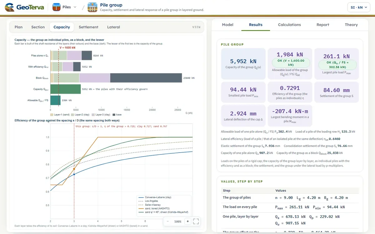
| One pile | 14.00 | 907.1 | 0.729 | 661.4 |
The spacing is the same in every row of the table, and the efficiencies differ because the soils do: the clay layers take the Converse–Labarre value for this grid, a sand layer the value of its kind of pile. The unit resistances f of the layers are worked out from the ground and the installation by the methods chosen for them in the Skin friction section, and the group effect is applied to what they give.
7Block failurethe group as a deep footing, layer by layer
With the piles close in a clay, the group can fail as a block: the piles and the soil between them move down together, shearing the soil along the perimeter of the group and bearing on the soil under its base. The source (after Terzaghi and Peck, 1967) takes the block as a deep footing of the length Lg, the width Bg of the outside of the outer piles and the depth L of the piles. Its capacity is the shear on the four faces plus the bearing under the base:
- The sides, in a clay layer. The soil shears against soil, not against the pile, so the shear stress is the undrained strength of the layer itself, τ = cu, not reduced by the adhesion factor of the single pile.
- The sides, in a sand layer. The source gives the block for a clay. For a sand layer the module takes the same reasoning with the friction of a granular soil: τ = K0 σ′v tan φ′, with K0 = 1 − sin φ′ (Jaky, 1944) and σ′v the mean effective stress over the length of the layer in the block. This is an extension beyond the source, and the sheet marks it.
- The base, on a clay. qb = cu(p) Nc*, cu(p) the strength of the clay under the base and Nc* the factor the source gives in a chart, which depends on L/Bg and Lg/Bg. The module reads the four curves of that chart, interpolates linearly in Lg/Bg between them and in Bg/Lg beyond 3, and keeps the value of L/Bg = 5 beyond the chart.
- The base, on a sand. The base of the block bears as the piles do, with the sum of their end bearing, n Qp.
| L / Bg | Lg/Bg = 1 | 2 | 3 | ∞ |
|---|---|---|---|---|
| 0.0 | 6.24 | 5.72 | 5.51 | 5.20 |
| 1.0 | 7.70 | 7.16 | 6.89 | 6.40 |
| 2.0 | 8.50 | 7.92 | 7.65 | 7.11 |
| 3.0 | 8.84 | 8.22 | 7.95 | 7.46 |
| 4.0 | 8.97 | 8.33 | 8.05 | 7.61 |
| 5.0 | 9.00 | 8.36 | 8.08 | 7.64 |
The capacity of the group is the lesser of the piles as individuals with their efficiencies (Section 6) and the block, and its allowable load is that capacity divided by the factor of safety entered:
| Layer | Soil | Length (m) | τ (kPa) | Shear on the faces (kN) |
|---|---|---|---|---|
| Layer-1 | sand | 4.00 | 9.3 | 624 |
| Layer-2 | clay | 6.00 | 50.0 | 5040 |
| Layer-3 | clay | 4.00 | 90.0 | 6048 |
| Base | cu(p) Nc* Lg Bg = 90 × 8.90 × 4.20 × 4.20 | — | — | 14126 |
| Block | 25838 |
8Elastic settlementa pile by Vesic’s three parts, and the group
A single pile settles by the shortening of its own length and by the compression of the soil it loads along the shaft and at the base. Vesic (1969) put the three parts together for a pile at its working load Qw, of which Qws is carried by the shaft and Qwp by the base:
The group settles more than one pile under the same load on each, because the stressed zone is that of the whole group. Vesic’s empirical relation for piles in sand takes the settlement of the group as that of one pile times the square root of the ratio of the width of the group to the width of a pile:
The working load of a pile is taken as V/n, and the module divides it between the shaft and the base in proportion to their ultimate resistances, Qs : Qp. For the worked group Qw = 177.8 kN, of which the shaft carries 132.9 kN and the base 44.9 kN; Ep = 30000 MPa, Es = 30 MPa, μs = 0.30. Then
| se1 (mm) | se2 (mm) | se3 (mm) | se of one pile (mm) | √(Bg/D) | Sg(e) (mm) |
|---|---|---|---|---|---|
| 0.21 | 2.46 | 0.34 | 3.00 | 2.646 | 7.94 |
9Consolidation settlementthe 2:1 spread from 2L/3, clay layer by clay layer
The clay layers under the group settle by consolidation, slowly and mostly. The source takes the load of the group to act on an equivalent footing of the size of the group at the depth 2L/3 below the top of the piles, as the piles have passed part of their load to the soil above that level, and to spread below it at 2 vertical to 1 horizontal. The stress the group adds at the middle of a clay layer, z below the level 2L/3, is
Every clay layer, or the part of it below 2L/3, then settles by the one-dimensional compression of its thickness H under its own mean stress. For a normally consolidated clay (σ′c = σ′o)
and for an over-consolidated one (σ′c = OCR σ′o), with the swelling index Cs (Cc/5 if none is entered) up to the preconsolidation stress and Cc beyond it:
The settlement of the group is the sum over the layers, Sc = ΣΔSi. The effective stress σ′o follows the layers and the water as entered, at the middle of the part of the layer below 2L/3.
| Layer | H (m) | z (m) | Δσ′ (kPa) | σ′o (kPa) | ΔS (mm) |
|---|---|---|---|---|---|
| Layer-2 | 0.67 | 0.33 | 77.9 | 106.5 | 23.4 |
| Layer-3 | 8.00 | 4.67 | 20.4 | 146.3 | 53.2 |
| Total | 76.7 |
10Lateral load: the p-multiplierswhy the rows share a load unequally, and the multipliers of the layers
A pile pushed sideways pushes on the soil in front of it, and the soil reacts along the pile — the p–y curve of the lateral module. When piles stand one behind another in the direction of the load, each pushes on soil that the pile in front of it has stressed and moved, so it finds less resistance there; and side by side the stressed zones overlap. Full-scale and centrifuge tests of groups (Brown, Morrison and Reese, 1988; McVay and others, 1995; Rollins and others, 2006) show that the p–y curve of a pile in a group keeps its shape but is lowered by a factor, the p-multiplier Pm, which depends on the row of the pile — the leading row, the second, the third and those behind — and on the spacing in the direction of the load.
The multipliers depend on the soil, and the module takes them by the soil of each layer. For a layer of clay it takes the equations Rollins and others (2006) fitted to full-scale tests of groups in stiff clay at spacings of 3.3 to 5.65 diameters:
For a layer of sand it takes the multipliers of AASHTO LRFD, which follow the tests of Brown, Morrison and Reese (1988) and the centrifuge tests of McVay and others (1995) at 3 and 5 diameters:
| Spacing in the direction of the load | Leading row | Second row | Third row and beyond |
|---|---|---|---|
| 3 D | 0.8 | 0.4 | 0.3 |
| 5 D | 1.0 | 0.85 | 0.7 |
| s / D | Clay: row 1 | row 2 | row 3+ | Sand: row 1 | row 2 | row 3+ |
|---|---|---|---|---|---|---|
| 3 D | 0.79 | 0.57 | 0.41 | 0.80 | 0.40 | 0.30 |
| 4 D | 0.86 | 0.72 | 0.58 | 0.90 | 0.63 | 0.50 |
| 5 D | 0.92 | 0.84 | 0.72 | 1.00 | 0.85 | 0.70 |
| 6 D | 0.97 | 0.93 | 0.83 | 1.00 | 0.90 | 0.80 |
| 7 D | 1.00 | 1.00 | 0.92 | 1.00 | 0.95 | 0.90 |
Layered ground
A pile in layered ground crosses clay and sand, and in the group each layer has its own multiplier: the p–y curve of the layer is scaled by the multiplier of the row for the soil of that layer. The same row therefore works at a different fraction of the single-pile resistance along its length. The multiplier depends on the spacing along the load and on the row; the module takes the spacing of the rows, sx, and the piles side by side along a row share the multiplier of their row.
The direction of the load
The leading row is the one the load pushes towards, the front of the group, and the rows are numbered from the front. If the lateral load reverses — wind, waves, an earthquake — every row is at times the leading one and at times in the lee. For a load that reverses the module gives every row the mean of the multipliers of the rows of the group.
11Solving the groupone deflection of the cap, rows of unequal load
The cap is rigid and held against turning, so every pile head has the same deflection Δ; the rows carry different loads because their p–y curves are scaled differently. The module therefore solves for the deflection at which the loads of the rows add up to the load on the cap:
A pile of row k is the single pile of the lateral module: the beam on non-linear springs solved by finite elements and Newton’s method (the Theory of that module), the p–y curves of its layers — those of Matlock (1970) for a clay layer and, for a sand layer, the criteria of API (2000) after Reese, Cox and Koop (1974) — scaled by the multipliers of row k for the soil of each layer. The cap is rigid, so the rows move together and the module controls the deflection, not the load: the head of the pile is held at a deflection and the load it takes is the reaction there, on a grid of deflections from a fraction of a millimetre to 4.9 pile widths, each solution the start of the next. The load–deflection curve of each kind of row — the leading row, the second, the third and beyond — is built in this way, and a curve that softens (a cyclic clay) is followed through its peak, which a load-controlled analysis cannot do. The sum of the curves, weighted by the piles in each row, is the load the group carries at each deflection; Δ is the first deflection at which it reaches H, found by bisection. Then every kind of row is solved again, exactly, at that Δ, and Δ is corrected by a secant step until the loads add up to H within two parts in a hundred thousand. The most the group can carry is the first peak of that sum, or its value at 4.9 pile widths if it has none; it does not depend on the load asked for. If the load is more than that the module says so and gives it.
For the worked group the cap deflects Δ = 2.92 mm under H = 900 kN. A pile of the leading row takes 135.3 kN, of the second row 89.6 kN and of the third 75.1 kN, against 100.0 kN for an equal share. A single pile carrying that equal share would deflect 1.85 mm, so the cap deflects 1.58 times as much as that single pile. Put the other way, a single pile would carry 154.8 kN at the deflection of the cap, and the piles of the group carry on average 0.65 of that — the efficiency of the group under the lateral load on the Results tab.
The engine of the single pile has been compared with an independent implementation written from the specification alone (14 piles, to within 0.01 % in the head deflection and in the largest moment; Theory of the lateral module), and the group is solved so that the loads of the rows add up to H to two parts in a hundred thousand.
The load P of a pile in the lateral analysis is the mean axial load V/n, which enters as the axial load of the lateral module (the P–δ effect). The axial loads from the moment on the cap (Section 2) are those of the statics of the rigid cap, and the lateral analysis runs on its own; the two are given together in the results. The bending moment and the deflection along the pile are given for every kind of row, and the largest moment of all is the one of the Results tab.
12Reading the resultswhat each result is, and the drawings
The Results tab gives:
- The largest and the smallest load on a pile, compression positive, from the moments on the cap, and the pile in tension if there is one, with the tension capacity of one pile and of the piles in tension together.
- The capacity of the group Qg(u) and its allowable load Qall, the group efficiency η, the capacity of one pile alone and of the block, and which governs; and beside the largest pile load the load one pile alone is allowed, Qu/FS.
- The settlement of the group: the elastic part, the consolidation part and their sum.
- The lateral response when a lateral load is entered: the deflection of the cap, the load a pile of the leading row takes, the largest bending moment in a pile of the group, the efficiency of the group under the lateral load, and the loads and moments of the rows.
The drawings follow the model before the analysis and give the numbers after it:
- Plan shows the piles, the cap and the loads, the rows numbered from the front, and after Analyze the load on every pile and the lateral load of each.
- Section shows the piles in the ground with the layers and the water table, the block, the level 2L/3 and the 2:1 spread, and after Analyze the unit shaft resistance of every layer and the stress at the middle of the clay layers.
- Capacity draws the piles as individuals, with and without the efficiency, and the block, each built of the layers it takes from, against the load; and the efficiency against the spacing.
- Settlement draws the stress at the middle of each clay layer and what the layer settles.
- Lateral draws the load–deflection curves of the rows, and the deflection and the bending moment along a pile of each kind of row.
The load on the group is judged against the allowable load of the group, and the largest pile load against Qu/FS (or against the allowable compression of one pile entered in the Design section, where that is the lesser). A pile in tension is judged against its tension capacity over the factor of safety (or the allowable tension entered, where that is the lesser), and the piles in tension together against their block. The settlement and the deflection of the cap are given beside the allowable values entered in the Design section and judged against them. The factor of safety on the capacity, for the group and for one pile, is the one in the Design section. Whether the settlement of the group is part of the analysis is chosen in the Settlement section: with it chosen, the elastic and the consolidation parts are worked out, drawn and judged; the loads on the piles, the capacity and the lateral response are worked out in either case. The load on every pile and the bending moment along a pile of each row are the loads for the structural design of the pile section.
13A worked exampleevery number computed by the module’s own code
The model the Model tab opens with: 9 bored piles in 3 rows of 3, D = 0.60 m, L = 14 m, at 1.80 m (3.0 D), in 4 m of sand, φ′ = 32°, then 6 m of clay, cu = 50 kPa, then 8 m of clay, cu = 90 kPa, with the water table 2 m down; V = 1600 kN, H = 900 kN, My = 900 kN·m. Every number below is computed by the module’s own code as this page opens.
The numbers of the worked group
- Loads on the piles (Section 2): 261.1 kN on the front piles to 94.4 kN on the back ones.
- Capacity (Sections 4 to 7): one pile alone Qu = 907 kN (678 shaft, 229 base); the group as individuals Qind = 5952 kN, η = 0.729; as a block Qblock = 25838 kN; so Qg(u) = 5952 kN and Qall = 1984 kN at FS = 3.0, against the V = 1600 kN carried.
- Settlement (Sections 8 and 9): elastic 7.9 mm + consolidation 76.7 mm = 84.6 mm.
- Lateral (Sections 10 and 11): the cap deflects 2.92 mm; the rows carry 406, 269, 225 kN, and the largest moment in a pile is 207 kN·m.
The same group with other choices
| Case | Qind (kN) | Qblock (kN) | Qg(u) (kN) | η | S (mm) | Δ (mm) |
|---|---|---|---|---|---|---|
| As entered | 5952 | 25838 | 5952 | 0.729 | 84.6 | 2.92 |
| Driven piles instead of bored | 6908 | 25838 | 6908 | 0.745 | 83.9 | — |
| Spacing 2.5 D | 5515 | 20490 | 5515 | 0.676 | 97.0 | 2.94 |
| Spacing 4 D | 6560 | 37982 | 6560 | 0.803 | 67.0 | 2.38 |
| Spacing 6 D | 7083 | 67656 | 7083 | 0.868 | 47.4 | 1.98 |
| The lateral load reverses | 5952 | 25838 | 5952 | 0.729 | 84.6 | 2.86 |
Moving the piles from 2.5 D to 6 D apart raises the capacity of the group from 5515 kN to 7083 kN, the group efficiency from 0.676 to 0.868, and lowers the cap deflection from 2.94 mm to 1.98 mm, as the p-multipliers rise towards 1. Driven instead of bored piles change the unit resistances of the layers (K = 1.4 K0 in the sand, the α of a driven pile in the clays) and the efficiency of a sand layer, which is 1 below φ′ = 40°: Qg(u) goes from 5952 kN to 6908 kN. With the lateral load reversing every row takes the mean multiplier and the cap deflects 2.86 mm instead of 2.92 mm.
14What the module assumesthe assumptions behind the numbers, in one place
Every analysis rests on assumptions. The module sorts them by how they reach the results:
- The group. A rectangular grid of vertical piles, or a triangular arrangement of them (at the corners of equilateral triangles, the rows s√3/2 apart and every second row shifted by s/2), of one section and length, under a rigid cap. In the triangular arrangement the lateral load acts across the rows, the p-multipliers follow the spacing of the rows and the shift of the rows does not enter them, and the efficiency is that of Converse and Labarre written over the neighbouring pairs, an extension of the source. The cap passes the load to the piles and adds nothing to their resistance: the passive pressure on it, the friction under it and the bearing of the soil under it are on the safe side.
- One pile. The resistance of a single pile is worked out by the methods of Section 3 — the K–δ method or that of Coyle and Castello in a sand layer, the α, λ or β method in a clay layer, Meyerhof, Vesic, Coyle and Castello or, for a bored pile in a clay, Reese and O’Neill at the base — for a driven, a bored or a jacked pile, and none of it is entered. The resistances are those of the ground as entered, around the pile as installed.
- The efficiency. The equations are empirical, from friction piles in clay; the sand rules are the chart of one series of tests (driven, never above 1) and the factors of AASHTO LRFD for bored shafts. The Converse–Labarre equation takes the spacing of each direction; the sand rules and the flag of 2.5 diameters take one spacing, the least distance between two piles. The Seiler–Keeney equation, with the spacing in feet, is given from 2 ft.
- The block. In a clay it is the footing of the source (after Terzaghi and Peck, 1967), with Nc* read from the curves of its chart. The shear in a sand layer, K0 σ′v tan φ′ on the faces, and the bearing of a block on sand as that of the piles, are the module’s extension of the source to layered ground. The base of the block bears on the layer it stands in, with the undrained strength of that layer in a clay.
- The loads. V is the load the piles carry, with the weight of the cap. The lateral load and the moments are at the base of the cap, and the loading is static or cyclic by the API reduction of the curves. A pile in tension takes its shaft resistance alone, a sand layer at three quarters of its resistance in compression; the weight of the pile, which resists uplift, is left out on the safe side.
- The settlement. An option of the Settlement section. The elastic settlement is by Vesic’s method for a pile in a uniform elastic soil, with one Es and one μs; the consolidation settlement is by the 2:1 spread of the source, a stress at the middle of each layer, at the end of consolidation. It is the settlement of the load of the group; a fill or a lowering of the water table is a loading of the ground of its own.
- The lateral response. The p-multipliers are those of tests in particular soils and at particular spacings (a stiff clay at 3.3 to 5.65 D, sand at 3 and 5 D); outside them the module interpolates and extrapolates as the section describes and flags a spacing below 3 D. The piles side by side along a row share the multiplier of their row. The cap is rigid and held against turning, and the axial loads from the moment are those of the statics of the rigid cap.
The methods of this module are the established ones of the literature and of current bridge specifications, put together layer by layer, and the numbers they give are to be set against the allowable values of the project.
15Referencesthe equations of the source and the p-multipliers
- Das, B.M. (2016). Principles of Foundation Engineering, 8th ed. Cengage Learning, Boston.
The resistance of one pile
- Meyerhof, G.G. (1976). Bearing capacity and settlement of pile foundations. Journal of the Geotechnical Engineering Division, ASCE, 102(GT3), 197–228.
- Vesic, A.S. (1977). Design of Pile Foundations. NCHRP Synthesis of Highway Practice 42, Transportation Research Board, Washington.
- Coyle, H.M. and Castello, R.R. (1981). New design correlations for piles in sand. Journal of the Geotechnical Engineering Division, ASCE, 107(GT7), 965–986.
- Mansur, C.I. and Hunter, A.H. (1970). Pile tests, Arkansas River project. Journal of the Soil Mechanics and Foundations Division, ASCE, 96(SM5), 1545–1582.
- Terzaghi, K., Peck, R.B. and Mesri, G. (1996). Soil Mechanics in Engineering Practice, 3rd ed. John Wiley & Sons, New York.
- Vijayvergiya, V.N. and Focht, J.A. (1972). A new way to predict capacity of piles in clay. Proceedings of the 4th Offshore Technology Conference, Houston, Paper OTC 1718.
- Burland, J.B. (1973). Shaft friction of piles in clay — a simple fundamental approach. Ground Engineering, 6(3), 30–42.
- O’Neill, M.W. and Reese, L.C. (1999). Drilled Shafts: Construction Procedures and Design Methods. FHWA-IF-99-025, Federal Highway Administration, Washington.
- Reese, L.C. and O’Neill, M.W. (1989). Drilled Shafts: Construction Procedures and Design Methods. FHWA-HI-88-042, Federal Highway Administration, Washington; the base of a drilled shaft in clay.
The group, the settlement and the lateral load
- Terzaghi, K. and Peck, R.B. (1967). Soil Mechanics in Engineering Practice, 2nd ed. John Wiley & Sons, New York.
- Kishida, H. and Meyerhof, G.G. (1965). Bearing capacity of pile groups under eccentric loads in sand. Proceedings of the 6th International Conference on Soil Mechanics and Foundation Engineering, Montreal, 2, 270–274.
- Vesic, A.S. (1969). Experiments with instrumented pile groups in sand. Performance of Deep Foundations, ASTM STP 444, 177–222.
- Jaky, J. (1944). The coefficient of earth pressure at rest. Journal of the Society of Hungarian Architects and Engineers, 7, 355–358.
- American Association of State Highway and Transportation Officials (2012). AASHTO LRFD Bridge Design Specifications, 6th ed.: the p-multipliers of pile groups and the resistance of shaft groups in cohesionless soil.
- Washington State Department of Transportation (2010). Bridge Design Memorandum No. 07-2010, Bearing resistance of shaft groups.
- Brown, D.A., Morrison, C. and Reese, L.C. (1988). Lateral load behavior of pile group in sand. Journal of Geotechnical Engineering, ASCE, 114(11), 1261–1276.
- McVay, M., Casper, R. and Shang, T.-I. (1995). Lateral response of three-row groups in loose to dense sands at 3D and 5D pile spacing. Journal of Geotechnical Engineering, ASCE, 121(5), 436–441.
- Rollins, K.M., Olsen, R.J., Egbert, J.J., Jensen, D.H., Olsen, K.G. and Garrett, B.H. (2006). Pile spacing effects on lateral pile group behavior: analysis. Journal of Geotechnical and Geoenvironmental Engineering, ASCE, 132(10), 1272–1283.
- Matlock, H. (1970). Correlations for design of laterally loaded piles in soft clay. Proceedings of the 2nd Offshore Technology Conference, Houston, Paper OTC 1204, 577–594.
- Reese, L.C., Cox, W.R. and Koop, F.D. (1974). Analysis of laterally loaded piles in sand. Proceedings of the 6th Offshore Technology Conference, Houston, Paper OTC 2080, 473–485.
- American Petroleum Institute (2000). Recommended Practice for Planning, Designing and Constructing Fixed Offshore Platforms — Working Stress Design, API RP 2A-WSD, 21st ed.
From theory to your own design
Analyse your own pile group in minutes
- The load on every pile, in compression and tension
- The efficiency, the block capacity and the allowable load
- Elastic and consolidation settlement, and the deflection of the cap
- A clean calculation report, saved as a PDF. Online: nothing to install, no dongle, on a phone, a tablet or a PC