
On this page · 24 chapters
- 1Slope stability, and this module
- 2The section
- 3The strength of the soil
- 4The factor of safety
- 5The slice
- 6Water in the ground
- 7Loads on the surface
- 8The ordinary method of slices
- 9The Bishop simplified method
- 10Spencer's method
- 11Which method
- 12The pseudo-static earthquake
- 13The tension crack
- 14The search for the critical circle
- 15Surfaces that are not circles
- 16Reinforcement
- 17Soil nails
- 18Ground anchors
- 19Geogrids
- 20Rock: the Hoek–Brown criterion
- 21A section from a DXF drawing
- 22The worked model, by the module
- 23What the module assumes, and what it does not do
- 24References
A slope fails when a mass of ground slides down a surface inside it. This page explains, section by section, how the module finds the factor of safety of such a surface by the method of slices — the section and its soils, the strength, the water, the loads, the ordinary method, Bishop's and Spencer's, the earthquake, the tension crack, the search for the critical surface, the soil nails, ground anchors and geogrids, the rock criterion — and closes with a model worked through by the module's own code, so that every number of the last section is one the program produces.
 PDF
Lecture slides
Ready-made slides for lectures and self-study
The mechanism, the derivation, the equations and the figures of this page, in teaching order. Every slide links back to its chapter.
1Slope stability, and this modulewhat the analysis answers, and the method
A slope fails when a mass of ground slides down a surface inside it. Whether it will is a question of balance: the weight of the mass, the water in it and the loads on it push it down the surface, and the strength of the soil along that surface holds it. Slope stability analysis puts a number on the balance — the factor of safety, FS, the ratio of what the ground can resist to what is needed to hold the mass still. FS above 1 means a reserve; FS = 1 is the limit; below 1 the mass would move (Figure 1).
The method is limit equilibrium by slices. The mass above a trial surface is taken as a rigid body that is just about to slide; the strength along the surface is used up to the same fraction everywhere, and that fraction is what FS measures. Nothing about the deformation of the slope is computed, and nothing about how the failure would start: the answer is a number for a surface, and the surface that gives the lowest number — the critical surface — is the one that matters.
- The section is drawn in layers between boundary lines, or read from a DXF drawing; each layer is given a soil. A soil is drained (c′, φ′), undrained (cu, φ = 0, which may grow with depth) or a rock mass (Hoek–Brown).
- Water: a groundwater line of any shape, water standing on the slope, a pore-pressure ratio ru, a rapid drawdown. Loads on the surface: strip and point loads in any direction. A pseudo-static earthquake. A tension crack at the crest.
- Reinforcement: soil nails, ground anchors and geogrids.
- Three methods of slices: the ordinary method, the Bishop simplified method and Spencer's method. The search: a grid of centres with a set of radii at each, refined around the best; surfaces that are not circles are searched too.
- The results: the factor of safety, static and pseudo-static, the critical surface, every slice with its forces, the working step by step, and a report.
The calculation is two-dimensional — plane strain: the section is one metre of an infinitely long slope, and every force is per metre of it. It is a design tool for the factor of safety of a surface, with the judgement of which surfaces, which strengths and which water left to the engineer; the last section says what it assumes and what it leaves out.
2The sectionprofiles, layers and soils
The module describes the section by profiles: the ground surface, the boundaries between the layers, the groundwater line and the base are each a line of straight pieces drawn from left to right — a function of x, z = g(x) (Figure 2). A vertical step is allowed; an overhang is not, because the ground would no longer have one height at each x.
- Coordinates: x to the right and z upward, in metres; forces per metre of the section. The slope may fall to the left or to the right: the sense of the sliding is found from the weights, and the slices keep their numbers, from the left, in the drawing, the tables and the report.
- Layers lie between the boundary lines, from the surface down: boundary k is the bottom of layer k, and the lowest layer rests on the base of the model. A boundary that rises above the one over it, or above the ground, is clipped there — the layer has no thickness where it happens.
- The base of the model is impenetrable: no slip surface goes below it. A stiff or rock layer can be given to the module as the base, so that circles stop on it.
- Soils are defined once and assigned to layers: a moist and a saturated unit weight (used above and below the groundwater line), and a strength (the next section). Colours and names are only for the drawing.
- Displayed values are rounded to the digits shown; the calculation is carried at full precision.
3The strength of the soildrained, undrained, undrained growing with depth
The shear strength of a soil on a surface depends on how hard the surface is pressed together. In terms of the effective stress σ′ = σ − u — the stress the grains carry — the strength of a drained soil is given by the Mohr–Coulomb envelope (Figure 3):
A saturated clay loaded faster than it can drain — a cut, an embankment on soft clay — carries the load partly on its pore water, and its strength is the undrained strength cu, independent of the normal stress, with φ = 0. It is described in total stress, so the pore pressure is not subtracted on a base in such a soil (it is taken as nil there). Many natural clays gain strength with depth; the module lets cu grow linearly:
The strength of a slice is read at the level of the middle of its base, where each base lies in one soil; every method and every kind of surface uses it. A rock mass has its own criterion, which is curved in this plane (Section 20). A soil is given one of the three descriptions; the choice — drained or undrained — is the engineer's, and it is the first assumption of the analysis: the short-term stability of a cut in soft clay is an undrained problem, its long-term stability a drained one.
4The factor of safetystrength over need, and the balance of moments about the centre
The factor of safety is the ratio of the shear strength the soil has to the shear stress it needs for equilibrium, taken as the same number all along the slip surface:
Reducing c′ and tan φ′ by the same factor until the mass is in equilibrium is how FS is found — the idea behind every method of this module. For a circular surface the equilibrium that decides is that of moments about the centre O (Figure 4): the weight of each slice turns the mass about O with the arm x − xc, and the shear force S on the base of a slice resists with the arm r, the radius, since it acts along the tangent.
The ratio is written as ΣR / ΣD, both sums in kN per metre, because dividing the moments by the radius gives forces that are easy to read. What the three methods of this module differ in is how they find N′, the effective normal force on each base, which the strength needs: the ordinary method from the weight alone, Bishop's from the vertical equilibrium of each slice, Spencer's from the equilibrium of forces and moments both.
5The slicegeometry, weight, base and forces
The mass between the slip surface and the ground is cut by vertical lines into slices, by their number or by a largest width. Every significant intersection of the geometry inside the mass is a mandatory side of a slice: the vertices of the ground surface and of the layer boundaries, the crossings of the boundaries with the ground and with the slip surface, the vertices of the water line and its crossings with the ground, the boundaries and the surface, and the ends of strip loads. In this way each base runs through one soil, and each slice carries one kind of load (the setting that drops these sides exists for hand checks only).
Every quantity of a slice is taken at its mid-ordinate, as in a hand calculation. The inclination of the base is that of the tangent of the arc there, α positive on the crest side of the centre — where the base falls toward the toe — and negative on the toe side:
The base takes the strength of the soil the arc runs through, c′ and φ′ or cu. The effective normal force is what presses the grains together: N′ = N − U, with U the pore force the water exerts on the base. A negative N′ would mean the base is in tension; the base can then carry no friction. In the ordinary and the Bishop methods N′ is held at zero, in Spencer's the friction of that base is left out and its cohesion kept; the loss is said in the results and marked on the drawing.
6Water in the groundpore pressure, standing water, ru and rapid drawdown
Water enters the analysis in three ways: as weight, because a saturated soil weighs more; as pore pressure on the base of every slice, which takes strength away; and, where it stands on the slope, as a load of its own (Figure 6).
The groundwater line
The water table is a line of any shape, drawn as the other lines of the model and read as level beyond its ends. Below it the pore pressure is hydrostatic:
No seepage is analysed, so a sloping water table is an approximation of the flow net. The weight of a slice takes the saturated unit weight below the line and the moist one above it, and the pore pressure is taken off the normal force on the base — a buoyant unit weight is never used beside it, so the water is counted once. Where the line stands above the ground there are two choices: it is held at the ground surface (the default: no water on the slope), or water stands on the slope — a reservoir, a canal, a river.
Water standing on the slope
Standing water presses on the ground normal to it. The vertical part of the pressure is the weight of the water over a slice; the horizontal part is a thrust into the slope, which acts at the centroid of the pressure over the rise of the ground in the slice:
The pore-pressure ratio
Where the pore pressure is known as a share of the overburden rather than from a line — a fill under construction, an embankment on soft clay — a soil is given a ratio ru. On a base in that soil:
Rapid drawdown
When the water against a slope falls faster than the soil can drain — a reservoir drawn down, a canal emptied — the support of the water is lost while the pore pressure stays. The water line of the model is the state before the drawdown; the drawdown takes it to a level zdd. The water standing on the slope above zdd is gone with its weight and thrust. A soil that does not drain stays saturated up to the old line, and the pore pressure on a base in it is the old one less the weight of the water taken off the ground above the point:
The factor of safety is that of the moment just after the drawdown, the lowest the slope sees; the full reservoir is analysed with the drawdown switched off.
7Loads on the surfacestrip and point loads, vertical, normal or inclined
A strip load q (kPa) runs along the ground surface between two positions s1 and s2, measured along the surface from its left end, so that it keeps its place when the ground is edited; a point load P (kN per metre of the section) stands at one position. A load has a direction (Figure 7): vertical, normal to the surface, or at an angle θ from the vertical.
Acting vertically or at an angle, a strip load is taken on the horizontal projection: on a piece of horizontal width b the force is q b, in the direction of the load. Acting normal to the surface, it is taken on the surface length: on a piece of length ℓ the force is q ℓ into the soil — its vertical part q b and its horizontal part q h. On a vertical face a load taken on the horizontal projection has no width and no effect, and a normal load is horizontal. Each slice carries the part of a load that falls between its sides, shared by horizontal width; a point load belongs to the slice that holds its point. The vertical loads add to the weight of the slice, the horizontal ones to the horizontal forces, whose moment about the centre enters the driving sum.
8The ordinary method of slicesFellenius: no forces between the slices
In the ordinary method of slices — Fellenius's, the Swedish method — the forces between the slices are neglected altogether. Each slice is then in equilibrium only in the direction normal to its base, which gives the normal force from the weight and the loads, and the factor of safety is the ratio of moments of Eq. (4):
With no water and no loads, in a homogeneous soil, it is the classic expression FS = Σ [c b / cos α + W cos α tan φ] / Σ W sin α. The method is simple and robust, and it is conservative: it takes no account of the forces the slices exert on each other, and its error grows with the depth of the circle and the pore pressure — on a deep circle in a soil with high pore pressure it can come out well under the other two methods (Section 11). A negative N′ is held at zero, as in every method of this module.
9The Bishop simplified methodvertical equilibrium of each slice, solved by iteration
In the Bishop simplified method the shear forces between the slices are still neglected, but every slice is put in vertical equilibrium, with the shear force on its base equal to the strength mobilised, (c L + N′ tan φ) / FS. Writing the vertical forces on a slice — the weight and the loads down, the vertical part of the normal and the shear force and of the pore force on the base — and solving for N′:
FS stands on both sides, because N′ depends on it through mα and the cohesion term; the equation is solved by iteration, starting from the value of the ordinary method (Figure 8). A few steps are enough, and the Calculations tab lists them. Bishop's method is the most used of the circular methods: it satisfies the equilibrium of moments and the vertical equilibrium of each slice, and it differs little from the methods that satisfy all of the equilibrium, on a circle.
Two guards are the usual ones of the method. A negative N′ is held at zero, and mα is not let fall under 0.2, which matters only on bases steeply inclined against the sliding, at the toe of deep circles; both are said when they happen.
10Spencer's methodforces and moments, with the forces between the slices parallel
Spencer's method satisfies both the equilibrium of forces and the equilibrium of moments. The forces between the slices are kept, taken parallel to one another: on every vertical side the shear force is a fixed fraction of the normal force,
Seen from the crest, with the mass sliding toward the toe and α positive when a base falls toward the toe, a slice carries the vertical force V (the weight, the vertical inertia force, the vertical load, the vertical part of a reinforcement), the horizontal force A toward the toe (the horizontal load, the thrust of standing water, the horizontal inertia force, the water in a tension crack, the horizontal part of a reinforcement), the normal force N and the shear force S = (c L + N′ tan φ) / FS on its base, and E and X on its two sides. Its two equations of equilibrium give the change of the normal force across the slice, ΔE = Ecrest − Etoe:
The sides at the two ends of the mass are free, so the forces add to nothing, ΣΔE = 0: this is the equilibrium of forces, and it gives a factor of safety FSf for every angle θ. The moments about the centre of the circle — N passes through it and the forces between the slices cancel — give a second one, FSm = Σ [c L + N′ tan φ] / Σ D, with the driving sum of the other methods. The two curves FSf(θ) and FSm(θ) cross at one angle: that angle and that factor of safety are the solution (Figure 9).
A reinforcement that is passive — a nail, a geogrid — is part of the resistance and is divided by FS in the equations of forces as it is in those of moments; an active one, an anchor, is a given force. The force of a reinforcement and the water of a tension crack act on the slice that holds the point where they meet the slip surface. A slice whose effective normal force comes out negative keeps its cohesion but loses its friction, and the denominator of ΔE is not let fall under 0.2 FS / cos θ.
When the solution is not admissible
The solution can be inadmissible — a tension between the slices, or an angle outside the ordinary range — and this is said. A slight tension, not more than 2 % of the largest force between the slices, is taken as numerical, a tolerance adopted by the program and not a rule of the method: it is noted and the solution stands. A larger one makes the solution inadmissible; the circle is then left out of the search, and the lowest factor of safety that Bishop's method gives on the circles left out is written beside the result, so that a lower circle is not hidden. On some circles the two curves do not meet at any angle; the search passes them over and gives their number. The line of thrust through the slices is not examined.
11Which methodwhat each satisfies, and how they compare
The three methods differ in what they satisfy and in what they neglect:
| Ordinary (Fellenius) | Bishop simplified | Spencer | |
|---|---|---|---|
| Moments about the centre | yes | yes | yes |
| Forces on each slice | normal to the base only | vertical | both directions |
| Forces between the slices | neglected | normal only (X = 0) | E and X = E tan θ |
| Unknowns | none: explicit | FS, by iteration | FS and θ |
| Surfaces | circles | circles | circles and polylines |
| Tendency | lowest, conservative | close to Spencer on a circle | the most complete |
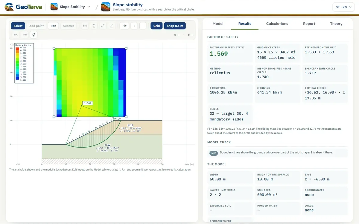
On the worked model of the last sections, on the same critical circle, the three give 1.569 (ordinary), 1.740 (Bishop) and 1.717 (Spencer): the ordinary method is the lowest, as it is nearly always, and the other two are close.
- The ordinary method is the one that can be checked by hand and is the cautious one; it is the default. Its result is the lowest of the three, markedly so on deep circles with high pore pressure, where its neglect of the forces between the slices matters most.
- Bishop's method is the usual choice for circular surfaces, and its result is within a few per cent of Spencer's on a circle.
- Spencer's method satisfies the full equilibrium and is the one for a surface that is not a circle. It is also the heaviest to compute, and on some circles it has no solution.
The method chosen on the Model tab is the one the circles are searched with; the factors of safety of the other two on the critical circle are given beside it for comparison.
12The pseudo-static earthquakeinertia forces at the centroid of each slice
The pseudo-static earthquake replaces the shaking by a steady acceleration, as a fraction of g, applied to the sliding mass (Figure 10). On every slice it puts the inertia forces of its soil mass Wsoil — the water ponded over a slice carries none — at the weight centroid of the slice, zg, found from the moist and the saturated parts of each soil in it:
The vertical force adds to the weight in every term. The moment of Fh about the centre of the circle, divided by the radius, adds to the driving sum; in the ordinary method its component normal to the base also changes the normal force:
The critical case tries both horizontal directions and both vertical ones and keeps the lowest factor of safety — an upward vertical force can be the more critical, since it lightens the mass and its normal force alike. The static and the pseudo-static factors of safety are both reported. The coefficients are the user's: the module applies them and does not derive them from a code; a reinforcement keeps the same force in the static and in the pseudo-static case.
13The tension crackits depth, and the water in it
A cohesive soil or a rock cannot carry tension at the crest, and a tension crack opens there. Its depth is that to which the soil stands in tension, as in Rankine's theory of the active state:
With the crack on, the slip surface of every circle ends, on the crest side, at the point where the sliding mass is as deep as the crack; from there a vertical crack runs up to the ground (Figure 11). The soil behind the crack is no part of the sliding mass, and the part of the arc inside the crack carries no strength. A circle whose mass is nowhere that deep is left whole.
Water standing in the crack to a height hw presses on the mass with the hydrostatic force, and its moment about the centre of the circle, divided by the radius, adds to the driving sum in all three methods:
A dry crack usually changes the factor of safety little, in either direction: it takes away the top of the mass, which drives, and the arc behind it, which resists. A crack full of water lowers it, and the water in a crack is the case that is the more often forgotten.
14The search for the critical circlea grid of centres, a set of radii, a refinement
The module does not analyse one circle but a whole family. The centres are the points of a rectangle laid over the slope, nx by nz; at every centre a set of radii is tried, equally spaced from the circle that just cuts into the ground to the one that touches the base of the model. Each circle is sliced and solved, and the centre keeps the lowest factor of safety it finds, with its radius:
On the worked model the grid is 15 × 15 centres with 12 radii at each: 4650 circles are tried, 3487 of them admissible. The lowest centre of the grid gives FS = 1.583; the refinement lowers it to 1.569 (Figure 12).
Two steps follow the grid. When its lowest centre stands on an edge of the rectangle the minimum may lie outside it, so the grid is carried on at the same spacing on that side, by a quarter of its points at a time, until the lowest centre stands inside it (or the grid has grown to 81 points across); the rectangle shown after the analysis is the one analysed. Then the search is refined: from each of the four lowest centres the centre and the radius are moved by half a spacing to the lowest of the neighbouring circles — the 26 neighbours in x, z and r — and the steps are halved whenever no neighbour is lower, down to a centimetre.
15Surfaces that are not circlesa polyline, Spencer about a point O, and its search
A slip surface need not be a circle: it may follow a weak layer, with a wedge down from the crest and one up to the toe. Such a surface is a polyline, from the left to the right like the ground surface, its two ends on the ground (Figure 13); it is carried on in a straight line along its first and its last piece to where it meets the ground, and the mass is the part where the ground lies above it. The surface has to cut the ground exactly twice and stay over the base of the model. Its vertices are sides of the slices, and the inclination of a base is that of the piece of the surface under the mid-ordinate of the slice.
The ordinary and the Bishop methods take their moments about the centre of a circle, where the normal forces of the bases have no arm; for a polyline they are not defined, and Spencer's method is the one used. Its equations of forces are those of a circle. The equation of moments is written about a point O — for a polyline a point over the toe end of the mass — where the normal force N of a base has the arm a, the shear force S the arm b, and the given forces their own:
Because the equations of force are satisfied at the solution, the moment about any point is the same equation: the solution does not depend on O, which is how it was checked. For a circle with O at the centre the arm of N is nil and that of S the radius, and the equation is the one of the circle; the sums R and D of the tables are the moments divided by an equivalent radius, the mean arm of the shear forces of the bases.
The search for the lowest polyline
The lowest surface is searched for as a polyline of n pieces. It starts from several surfaces — the one drawn, a polyline along the critical circle, and for each layer boundary one that goes down from the crest at 60°, follows the boundary and comes up to the ground beyond the toe at 25° — and every start is moved vertex by vertex, in x and in z, and in groups (all the interior vertices up or down, their depth under the chord scaled), by steps that halve when no move lowers the factor of safety. A move is kept only when the surface stays admissible: under the ground and over the base, inside the width of the model, no piece steeper than 85°, and — when the box is ticked — convex as seen from the mass, the angle of the pieces falling from the crest to the toe never growing again, which keeps the search from the zigzag surfaces that are low only because they are not kinematically possible. A weak layer shows as a surface that follows it; where there is none, the polyline comes close to the circle, a little under it.
16Reinforcementthe force across the surface, passive and active
A reinforcing element is a line in the section that carries a tension across the slip surface. For every circle the point where the element crosses the arc is found; the length from the head to the crossing is Lf, in front of the slip surface, and the bonded length beyond it Lb, behind it. An element whose inner end lies inside the sliding mass, or whose head lies outside it, carries nothing on that circle. The force Tm per metre of the section acts on the sliding mass at the crossing, along the element, toward its inner end (Figure 14).
The moment of the force about the centre of the circle, divided by the radius and counted positive against the sliding, is:
A passive element — a nail, a geogrid — works as the mass moves, and its moment is added to the resisting side. An active element — an anchor — carries its load before the mass moves, and its moment is taken from the driving side:
For the same force an active element therefore raises the factor of safety more than a passive one. The effect of the force on the normal force at the base of the slices is neglected, which is on the safe side, and the force is the same in the static and the pseudo-static case. Because the circles of the grid are free, the critical circle with reinforcement is the lowest of those that cut the elements and those that pass beyond their ends; it usually moves deeper, and the rectangle of centres may have to be enlarged.
17Soil nailstension of the bar, pull-out either side of the surface
A soil nail is a bar grouted in a drill hole, its head on the ground surface, inclined below the horizontal into the slope (Figure 15). It has a length L, the tensile capacity of the bar Tt, the ultimate bond stress qu between the grout and the soil on a drill hole of diameter Dh, the capacity of its head — the facing — Th when it has one, and a spacing Sh along the slope, out of the plane of the section. The force it carries across the slip surface is the least of three:
The nail is passive: it works as the mass moves. Its force is divided by the spacing, since the section is one metre of the slope and the nails stand Sh apart. The shear and the bending of the bar, and the weight of the nail, are not counted. A nail whose head is outside the circle, or whose tip is inside the mass, carries nothing on that circle.
18Ground anchorslock-off load, free length and root
A ground anchor is a tendon with a free length Lfree from its head and a grouted root behind it, stressed and locked off at a load P. The free length carries no bond; the root holds the anchor. Across a slip circle the anchor carries the least of three:
Lb is the whole root when the circle crosses the free length, and the part of the root behind the crossing when the circle cuts the root. The anchor is active: the load is in the tendon before the mass moves, so its moment is taken from the driving side of Eq. (27). An anchor is a given force in the equations of Spencer's method; it is not divided by FS there.
19Geogridsdesign strength, pull-out and the connection
A geogrid is a horizontal sheet laid in the soil from the ground surface inward, continuous along the slope (Figure 16). It has a length L, a long-term design strength Td per metre of the section — the strength left after the reductions for creep, damage and durability — an interaction coefficient Ci between the soil and the geogrid, and, when it is fixed to a facing, the strength of that connection Tc. Its pull-out resistance per metre of length comes from the friction on its two faces under the effective overburden σ′v:
σ′v is the weight of the soil above the sheet — saturated below the water table — less the pore pressure; the loads on the surface are left out, on the safe side. The geogrid is passive, and acts along the sheet. Because a geogrid is laid in layers, the module can place a whole row of them at a given spacing.
20Rock: the Hoek–Brown criteriona curved envelope, and its tangent at every base
A rock mass is given by the uniaxial compressive strength of the intact rock σci, the Geological Strength Index GSI, the constant of the intact rock mi and the disturbance factor D (0 for an undisturbed mass, 1 for a heavily blasted or relaxed one). The generalised Hoek–Brown criterion is written in the principal stresses:
The method of slices needs the shear strength on the base of a slice under its normal stress, so the criterion is turned into its envelope in the τ–σ′n plane (Balmer's relations). With d = dσ′1 / dσ′3, a point of the envelope is:
and the tangent to the envelope there gives the instantaneous friction angle and cohesion (Figure 17):
For this mass the criterion gives mb = 0.6567, s = 0.00042 and a = 0.5223; the strength under σ′n = 200 kPa is τ = 207.6 kPa.
On a base in rock the effective normal stress is σ′n = N′ / L; the σ′3 that belongs to it is found, and the resistance of the base is R = τ L = ci L + N′ tan φi. Every base has its own c and φ; they are listed in the slice table. In the ordinary method N′ is known before the strength; in the Bishop method N′ depends on c and φ, and the three are found together on every base at every step. Where the normal force of a base comes out negative the base has no normal stress to carry: in the ordinary and the Bishop methods it is held at zero, and in Spencer's method, after the unconstrained solution, the friction of the base is left out and its strength is that of the envelope at zero normal stress, τ = c. Below the tensile strength of the mass, σt = −s σci / mb, there is no strength.
21A section from a DXF drawingthe layers, and what each becomes
A section drawn in a CAD program is read by its layers; the names are read without regard to capitals, spaces, hyphens and underscores (Figure 18).
- EXTERNAL — the outer boundary of the section as one closed line: the ground surface, the two sides and the base. Its upper chain becomes the ground surface and its lowest level the base of the model.
- MATERIAL — the lines between the soils. A line that ends inside the section is carried on along the ground surface, so that the soil above it is absent there; every region between two boundaries gets a soil of its own.
- WATER TABLE — the groundwater line.
- NAIL, ANCHOR, GEOGRID — the reinforcement, one line for each element. The end nearer the ground surface is the head, which is put on the surface at its x; the direction, the inclination and the length come from the line. An anchor drawn with three points — head, end of the free length, tip — or as two lines end to end gives its free length and its root; drawn as a single line, 45 % of its length is taken as free. A geogrid is taken horizontal, with the horizontal length of its line.
A line that falls outside the section is not read, and the elements are named from the top down. What the drawing leaves out — the unit weights and strengths of the soils, the capacities of the elements, the loads and the earthquake — is entered on the Model tab. There, the button DXF format & examples… beside Import DXF… gives these notes with the other names that are read for each layer, and three example drawings to download — a slope with a water table, a cut held by soil nails and a ground anchor, an embankment with geogrids — each of which Import DXF… reads as it is.
22The worked model, by the moduleevery number computed by the module's own code
The model the Model tab opens with is a 10 m slope at 2 horizontal to 1 vertical, rising to the right: the ground goes through (0, 0), (10, 0), (30, 10) and (50, 10), the base of the model lies at z = −6 m, and the layers are fill above the level z = 4 m (γ = 18.0 kN/m³, c′ = 5 kPa, φ′ = 30°) over clay below it (γ = 17.5 kN/m³, c′ = 20 kPa, φ′ = 18°). There is no water, no load and no earthquake, and the method is the ordinary one. Every number below is computed by the module's own code as this page opens.
The search over the grid Figure 12 finds a critical circle with its centre at (16.52, 16.08) and a radius of 17.35 m. It cuts the ground at x = 10.00 m, at the toe, and at x = 32.77 m on the crest, and the mass between is cut into 33 slices — Figure 19.
One slice, by hand
Slice 22 is the heaviest. Its width is b = 0.759 m and its middle is at xm = 24.800 m; the arc runs through the clay there, c′ = 20 kPa, φ′ = 18°. With Eq. (5) and Eq. (6):
Every slice, and the sums
| Slice | b (m) | α (°) | W (kN/m) | L (m) | Soil | c′ (kPa) | φ′ (°) | N′ (kN/m) | R (kN/m) | D (kN/m) |
|---|---|---|---|---|---|---|---|---|---|---|
| 1 | 0.00 | −22.1 | 0.0 | 0.00 | clay | 20 | 18 | 0.0 | 0.0 | −0.0 |
| 5 | 0.76 | −12.9 | 28.7 | 0.78 | clay | 20 | 18 | 28.0 | 24.7 | −6.4 |
| 9 | 0.76 | −2.7 | 54.4 | 0.76 | clay | 20 | 18 | 54.4 | 32.9 | −2.6 |
| 13 | 0.35 | 5.5 | 32.2 | 0.35 | clay | 20 | 18 | 32.0 | 17.4 | 3.1 |
| 17 | 0.76 | 15.0 | 82.7 | 0.79 | clay | 20 | 18 | 79.9 | 41.7 | 21.4 |
| 21 | 0.76 | 25.7 | 88.5 | 0.84 | clay | 20 | 18 | 79.7 | 42.8 | 38.4 |
| 22 | 0.76 | 28.5 | 88.5 | 0.86 | clay | 20 | 18 | 77.8 | 42.5 | 42.2 |
| 25 | 0.76 | 37.5 | 84.4 | 0.96 | clay | 20 | 18 | 67.0 | 40.9 | 51.4 |
| 29 | 0.27 | 50.3 | 23.7 | 0.42 | fill | 5 | 30 | 15.2 | 10.8 | 18.2 |
| 33 | 0.76 | 66.2 | 12.7 | 1.88 | fill | 5 | 30 | 5.1 | 12.4 | 11.6 |
| Σ | 1841.1 | 1613.8 | 1006.3 | 641.3 |
The same circle by the other two methods
Bishop's method starts from this value and iterates Eq. (14): 1.5690 → 1.7232 → 1.7385 → 1.7399 → 1.7401 → 1.7401 → 1.7401 → 1.7401, converged after 7 steps (Figure 8). Spencer's method finds the angle at which the two curves of Figure 9 cross:
| Method | FS | Σ resisting (kN/m) | Σ driving (kN/m) | Note |
|---|---|---|---|---|
| Ordinary (Fellenius) | 1.569 | 1006.3 | 641.3 | explicit |
| Bishop simplified | 1.740 | 1116.0 | 641.3 | 7 iterations |
| Spencer | 1.717 | 1101.2 | 641.3 | θ = 18.54° |
What each addition does
Each of the following is added to the model alone, the critical circle is searched again, and the three methods are given on it (the earthquake is the pseudo-static case with the critical direction). The numbers are the module's own:
| Model | Ordinary | Bishop | Spencer |
|---|---|---|---|
| The model as it opens (static) | 1.569 | 1.740 | 1.717 |
| + a water table rising into the slope | 1.255 | 1.568 | 1.564 |
| + a strip load of 20 kPa, x = 25 to 32 m | 1.400 | 1.585 | 1.556 |
| + the earthquake, kh 0.15, kv 0.05 (critical) | 1.138 | 1.265 | 1.250 |
| + four soil nails, 14 m long | 1.753 | 2.018 | 2.031 |
23What the module assumes, and what it does not dothe assumptions and the limits in one place
Every calculation rests on assumptions. The module sorts them by how they reach the results:
- The model — plane strain, one metre of an infinitely long slope; the strength of each soil is the one given and is the same in every direction (except the rock criterion, which is isotropic); the soil is rigid until the surface moves; the ground, the boundaries and the water are profiles of x.
- The water — hydrostatic under a line, or a ratio ru of the overburden: no seepage is analysed. A rapid drawdown takes the pore pressure to follow the whole change of the load (B̄ = 1) and the drawdown as instant; a partly drained state between the two is not analysed.
- The slices — every quantity at the mid-ordinate; a negative effective normal force is held at zero (the friction of that base is left out in Spencer's method); the earthquake is pseudo-static, with coefficients the user gives, and the standing water carries no inertia.
- The methods — the ordinary method neglects all forces between the slices, Bishop's the shear forces, and Spencer's takes the forces between them parallel with one angle for the whole mass; the equilibrium of moments is satisfied by all three, that of forces by Spencer's alone. Morgenstern–Price and Janbu methods are not offered. The line of thrust through the slices is not examined.
- The tension crack has one depth for all circles and is vertical; the force of the water in it does not change the normal force on the bases.
- The reinforcement — a force at the crossing, along the element; it does not change the normal force on the base and does not change with the earthquake; the shear and the bending of a nail are not counted; the loads on the surface are not counted in the overburden that holds a geogrid.
- The search finds a lowest surface near its starts, not a proof of the lowest of all: the circles by a grid with a refinement; a surface that is not a circle is a convex polyline of a fixed number of pieces, found from a few starting surfaces, and the ordinary and the Bishop methods do not apply to it.
- The rock by the Hoek–Brown criterion is the same in every direction; sliding on a single joint set, on a plane or a wedge, is not analysed, and the disturbance factor is one value for the whole rock.
A circle may also be passed over: one that cuts the ground more than twice (through a berm), that passes below the base, or whose mass is nowhere half a metre deep. Where a message is raised the results say what was assumed and what was found; the screen may suggest what to do next, the report only states.
What the module does not do
- Three-dimensional effects — the end of a slide, the width of a slope, the corner of an excavation.
- Deformation — how far the slope moves, and how a failure would start (progressive failure, strain softening).
- Seepage and consolidation — the pore pressure is given, not computed; its dissipation with time is not followed.
- Dynamic analysis — Newmark displacements and a time history of the shaking; the pseudo-static case is a check, not a prediction.
- A verdict — the factor of safety is given; what factor is enough is the engineer's and the standard's.
24Referencesthe methods, the criterion and the reinforcement
- Fellenius, W. (1936). Calculation of the stability of earth dams. Transactions of the 2nd Congress on Large Dams, Washington, 4, 445–463.
- Bishop, A.W. (1955). The use of the slip circle in the stability analysis of slopes. Géotechnique, 5(1), 7–17.
- Spencer, E. (1967). A method of analysis of the stability of embankments assuming parallel inter-slice forces. Géotechnique, 17(1), 11–26.
- Morgenstern, N.R. and Price, V.E. (1965). The analysis of the stability of general slip surfaces. Géotechnique, 15(1), 79–93.
- Duncan, J.M., Wright, S.G. and Brandon, T.L. (2014). Soil Strength and Slope Stability, 2nd ed. Wiley.
- Terzaghi, K. (1950). Mechanism of landslides. In Application of Geology to Engineering Practice (Berkey Volume), Geological Society of America, 83–123.
- Rankine, W.J.M. (1857). On the stability of loose earth. Philosophical Transactions of the Royal Society of London, 147, 9–27.
- Hoek, E., Carranza-Torres, C. and Corkum, B. (2002). Hoek–Brown failure criterion — 2002 edition. Proceedings of the 5th North American Rock Mechanics Symposium, Toronto, 1, 267–273.
- Balmer, G. (1952). A general analytical solution for Mohr's envelope. Proceedings ASTM, 52, 1260–1271.
- Lazarte, C.A., Robinson, H., Gómez, J.E., Baxter, A., Cadden, A. and Berg, R. (2015). Soil Nail Walls — Reference Manual. Geotechnical Engineering Circular No. 7, FHWA-NHI-14-007.
- Sabatini, P.J., Pass, D.G. and Bachus, R.C. (1999). Ground Anchors and Anchored Systems. Geotechnical Engineering Circular No. 4, FHWA-IF-99-015.
- Berg, R.R., Christopher, B.R. and Samtani, N.C. (2009). Design and Construction of Mechanically Stabilized Earth Walls and Reinforced Soil Slopes. Geotechnical Engineering Circular No. 11, FHWA-NHI-10-024.
From theory to your own design
Find the factor of safety of your own slope in minutes
- The critical circle and its factor of safety, with the forces on every slice
- Groundwater, surface loads, an earthquake, soil nails, ground anchors and geogrids
- Static and pseudo-static cases
- A clean calculation report, saved as a PDF. Online: nothing to install, no dongle, on a phone, a tablet or a PC