
On this page · 10 chapters
The bearing-capacity theory of Richards, Elms and Budhu for a continuous footing under static and earthquake loading, derived step by step: Coulomb’s active and passive wedges, the factors Nq, Nγ and Nc, the pseudo-static earthquake with the Mononobe–Okabe coefficients, and how much of the capacity an earthquake takes away. The figures are drawn to scale from the equations.
 PDF
Lecture slides
Ready-made slides for lectures and self-study
The mechanism, the derivation, the equations and the figures of this page, in teaching order. Every slide links back to its chapter.
1Scope and assumptionsTwo Coulomb wedges, static and earthquake loading.
Richards, Elms and Budhu (1993) proposed a bearing-capacity theory for a continuous footing that can be applied under earthquake loading. Instead of the log-spiral mechanism of Terzaghi or Meyerhof it uses a simplified failure surface made of two Coulomb wedges, which gives every bearing-capacity factor in closed form — for the static case and, with the Mononobe–Okabe coefficients, for the seismic case. This page follows the presentation of the source. The module assumes:
- A continuous (strip) footing of width B at the depth Df; the soil above the base acts as the surcharge q = γDf only.
- A homogeneous c–φ soil with φ > 0 and no water table in the failure zone.
- The earthquake as a pseudo-static body force: the horizontal and vertical seismic coefficients kh, kv act on the soil wedges and on the loads.
- The wall friction on the vertical face between the two wedges δ = φ/2, as the authors suggest.
2The static failure surfaceCoulomb’s active and passive wedges and their angles.
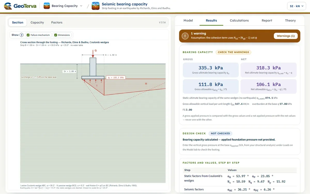
Under the footing the soil fails as Coulomb’s active wedge ABC: the footing pushes it down and it pushes the soil beside it sideways. That soil fails as Coulomb’s passive wedge BCD. The two meet on the vertical face BC, of height H, where the wall friction δ acts. The slip planes AC and CD make the angles αA and αP with the horizontal — the angles of the critical Coulomb wedges:
The forces on the wedges per unit length of the footing (Figure 1 b) are the Coulomb active and passive forces PA, PP on BC, the resultants RA, RP on the slip planes, and the weights WI, WIII. The horizontal components of the Coulomb forces use the coefficients
3The surcharge term — NqThe horizontal balance on BC with a surcharge only.
Take the surcharge alone (φ ≠ 0, γ = 0, q ≠ 0): the footing pressure is q′u. The horizontal forces on BC balance,
and with a uniform surcharge each is the pressure coefficient times the surcharge times the height H: q′u on the active side, q on the passive side,
so that
4The self-weight term — NγThe same balance with the weight of the wedges.
Now the weight alone (φ ≠ 0, γ ≠ 0, q = 0): the footing pressure is q″u. On the active side it acts as a surcharge on top of the weight of the wedge, on the passive side only the weight acts:
Equating the two,
The height of the face BC follows from the active wedge, H = B tan αA, and
5The static bearing capacitySuperposition, Nc, and the static factors.
With the surcharge and the weight together, the two parts are added (superposition):
For the cohesion, a Coulomb wedge analysis at φ = 0 gives Nc = 6; for brevity the authors use the familiar relation
and the ultimate bearing capacity of a continuous footing on a c–φ soil is
| φ (°) | δ (°) | αA (°) | Nq | Nγ | Nc |
|---|---|---|---|---|---|
| 5 | 2.5 | 42.22 | 1.53 | 0.49 | 6.11 |
| 10 | 5.0 | 45.19 | 2.37 | 1.38 | 7.77 |
| 15 | 7.5 | 48.13 | 3.70 | 3.02 | 10.09 |
| 20 | 10.0 | 51.06 | 5.90 | 6.06 | 13.46 |
| 25 | 12.5 | 53.97 | 9.67 | 11.92 | 18.59 |
| 30 | 15.0 | 56.86 | 16.51 | 23.76 | 26.86 |
| 35 | 17.5 | 59.74 | 29.89 | 49.52 | 41.26 |
| 40 | 20.0 | 62.60 | 59.03 | 111.96 | 69.16 |
| 45 | 22.5 | 65.45 | 133.87 | 290.89 | 132.87 |
6Earthquake loadingThe pseudo-static wedges, θ, and the Mononobe–Okabe coefficients.
Under an earthquake the same two wedges are analysed with pseudo-static inertia forces (Figure 2). The resultant of the gravity and inertia forces is tilted from the vertical by
The critical wedges now make the angles
and the horizontal earth-pressure coefficients become the Mononobe–Okabe coefficients:
The equilibrium is the same as in the static case, so the factors keep their form:
At θ = 0 every seismic expression returns to its static form.
7How much the earthquake takes awayThe seismic factors as fractions of the static ones.
The source gives these reductions as charts after Richards et al. (1993); Figure 3 draws them from the closed forms. The earthquake reduces the self-weight term most: at tan θ = 0.2 NγE is about a third of Nγ, while NqE and NcE keep about half of their static values.
The limit θ = φ
As θ approaches φ the active wedge flattens (α = φ − θ → 0) and all three seismic factors fall towards zero: the frictional soil has no reserve left against the horizontal acceleration. The theory therefore holds only while kh/(1 − kv) < tan φ, and the module stops when θ ≥ φ. The same critical ratio kh/(1 − kv) is where the theory predicts the seismic settlement of the footing to begin.
8Allowable pressure and the checkFrom the seismic capacity quE.
The module takes the allowable pressures from the seismic capacity quE, keeping the gross and the net pressures apart, and reports the static qu beside it:
The applied pressure qapplied is the vertical gross pressure at the base (V/A per unit length, V/B) of the earthquake load case. The footing passes when qapplied ≤ qall,g (FSactual = quE/qapplied) and qapplied − q ≤ qall,n. The allowable load per unit length is Qall = qall,g·B.
9Worked exampleThe module’s opening model, computed live.
A continuous footing B = 1.5 m at Df = 1 m; γ = 17 kN/m³, φ = 25°, c = 30 kPa; kh = 0.25, kv = 0 (the module’s opening model).
The earthquake takes the ultimate bearing capacity from 874.14 kPa to 335.28 kPa, to 38% of the static value.
10ReferencesSources of the theory.
- Richards, R., Elms, D.G. and Budhu, M. (1993). Seismic bearing capacity and settlements of foundations. Journal of Geotechnical Engineering, ASCE, 119(4), 662–674.
- Das, B.M. (2017). Shallow Foundations: Bearing Capacity and Settlement, 3rd ed. CRC Press — Section 6.3.1; this page follows the order of its derivation.
- Mononobe, N. and Matsuo, H. (1929). On the determination of earth pressures during earthquakes. Proc. World Engineering Congress, Tokyo, 9, 177–185.
- Okabe, S. (1926). General theory of earth pressure. Journal of the Japanese Society of Civil Engineers, 12(1).
The figures are drawn to scale from the equations of this page.
From theory to your own design
Find the seismic capacity of your own footing in minutes
- The static and the seismic capacity side by side, with their factors
- The loss of capacity caused by the earthquake
- The wedge geometry drawn on the section
- A clean calculation report, saved as a PDF. Online: nothing to install, no dongle, on a phone, a tablet or a PC