
On this page · 10 chapters
A pile seldom passes through one soil. This page is about the bookkeeping that follows: which rule applies over which stretch of the shaft, what the effective stress is once the layers above have been counted, and which layer the point belongs to.
 PDF
Lecture slides
Ready-made slides for lectures and self-study
The mechanism, the derivation, the equations and the figures of this page, in teaching order. Every slide links back to its chapter.
1A pile through several layersEach layer answers with its own rule.
A pile rarely passes through one soil. This module takes the profile as it is: up to four layers, each described as a sand or as a clay, and applies to every layer the rule that belongs to its own material. The capacity is still the two familiar parts, but each is now assembled rather than read off a single formula.
Nothing here is new theory. The sand rules are those of the sand module and the clay rules those of the clay module; what this module adds is the bookkeeping — which rule applies over which stretch of the shaft, and what the effective stress is at each depth once the layers above have been accounted for.
2Effective stress through the layersContinuous stress, stepped friction.
The effective vertical stress is what ties the layers together. It accumulates downwards through every layer above the depth in question, with the moist unit weight above the water table and the submerged unit weight below it — so a clay layer, which contributes nothing of its own strength to a sand layer, still changes what that sand layer offers by the weight it adds:
The friction, by contrast, is not continuous. At a sand–clay boundary the rule itself changes, and the unit friction can jump up or down by a wide margin — that step is real, not an artefact of the calculation, and it is the clearest signature of a layered profile.
3The point takes its own layerThe method chosen for the tip’s own soil.
The point resistance belongs to one layer only: the one the tip is embedded in. The module finds that layer, applies the method chosen for its own material, and reports which one it used.
A sand tip
For a sand c′ = 0, so only the surcharge term survives and the unit point resistance is the effective vertical stress at the tip times a pile factor. Three routes are offered, exactly as in the sand module. Meyerhof reads N*q from the friction angle of the tip layer and caps the result:
with pa the atmospheric pressure (100 kN/m²). N*q comes from the friction angle of the tip layer, read from Meyerhof’s chart:
Vesic takes the mean effective stress at the tip and a factor built from the rigidity index of that layer, so the stiffness of the sand enters as well as its strength; it needs m = Es/pa. Coyle & Castello read N*q off their own field chart against the embedment ratio L/D and the friction angle, with no cap — the module fills that box in from the chart at the tip layer’s φ′ and lets you type over it:
A clay tip
In a saturated clay under undrained conditions the friction angle is zero and the point resistance is a multiple of the undrained strength of the tip layer alone. Meyerhof takes the classical nine; Vesic builds the factor from the rigidity index of the clay instead, which in undrained loading reduces to a closed form in cu:
A bored pile whose tip sits in clay is offered a third route, Reese and O’Neill’s drilled-shaft expression, which works from the clay beneath the base rather than from the strength at the tip alone; it has a section of its own below, since the same procedure also changes what the shaft is credited with.
Coyle & Castello is a sand correlation and has no meaning at a clay tip; choosing it there leaves the clay rule in force and the module says so in the warnings.
The effective stress at the tip is built from every layer above it, so the layers still matter to a sand tip through q′ — and not at all to a clay tip.
4The rules over a sand layerK–δ or Coyle & Castello, per layer.
Over a sand layer the shaft resists by friction against the horizontal effective stress, and the layer carries its own numbers: the module asks for a method, a K and a δ′ for each sand layer.
The K–δ method
The unit friction is the earth-pressure coefficient K times the effective vertical stress, times the friction of the pile–soil interface:
In reality K varies with depth — roughly the Rankine passive coefficient at the top of the pile, and possibly below the at-rest coefficient deeper down — so an average is recommended for each kind of pile, and it follows the installation:
| Pile type | K |
|---|---|
| Bored or jetted | ≈ Ko = 1 − sin φ′ |
| Low-displacement driven | ≈ Ko to 1.4Ko |
| High-displacement driven | ≈ Ko to 1.8Ko |
The critical depth applies to the whole pile, not to each sand layer separately: below L′ = 15D the effective stress used for the friction is held at its value at L′, wherever the layer boundaries happen to fall. A sand layer deep in the profile therefore contributes a constant unit friction over its whole thickness.
Coyle & Castello
The alternative offered for a sand layer pairs a chart-read K with δ′ = 0.8φ′ and the mean effective stress of that layer, with no critical depth at all — the averaging plays that part:
5The rules over a clay layerα, λ or β, per layer.
Over a clay layer the shaft resists by adhesion or by effective stress, and again the layer carries its own choice and its own numbers. All three routes of the clay module are offered.
The α method
The unit friction is a fraction α of the undrained strength of that layer, with α read from a published correlation that falls as the clay gets stronger:
| cu/pa | α |
|---|---|
| ≤ 0.1 | 1.00 |
| 0.2 | 0.92 |
| 0.3 | 0.82 |
| 0.4 | 0.74 |
| 0.6 | 0.62 |
| 0.8 | 0.54 |
| 1.0 | 0.48 |
| 1.2 | 0.42 |
| 1.4 | 0.40 |
| 1.6 | 0.38 |
| 1.8 | 0.36 |
| 2.0 | 0.35 |
| 2.4 | 0.34 |
| 2.8 | 0.34 |
The λ method
One coefficient applied to a combination of the effective stress and the undrained strength, with λ read from the table against the embedded length of the pile:
Vijayvergiya and Focht wrote λ as one average over the whole embedded length of a pile in clay. Applying it to a single layer of a mixed profile — λ at the pile’s own length, with that layer’s mean effective stress and its own strength — is an extension of the method by this program, not part of it; the module says so wherever the number appears.
The β method
The effective-stress approach of Burland, with the overconsolidation adjustment after Meyerhof. The undrained strength drops out entirely and the friction follows the vertical effective stress through the remoulded drained friction angle of that layer (c′ = 0). At any depth in such a layer,
with K taken conservatively at rest and raised for an overconsolidated layer by √OCR. The two combine into one expression, which at OCR = 1 reduces of itself to the normally consolidated form — there are not two rules:
φ′R and OCR are entered, not correlated: the source defines the remoulded drained friction angle but gives no relation to read it from, so nothing is filled in from the ground. Each φ′R box opens at 30° and each OCR box at 1, to be replaced with the values that belong to these clays.
Because f follows σ′(z), the unit friction grows with depth inside a β layer and steps where β changes at a boundary. The layer average f̄ = βσ̄′ is what gives that layer’s share of Qs, since βσ̄′ΔL is the integral of βσ′(z) over it — and the mean is the true integral over the layer, not the average of its two ends, a distinction that matters as soon as the water table crosses it.
The unit friction of an α layer does not depend on depth at all: it is one number for the layer, which is why the friction profile of a mixed pile is flat over each α stretch and sloping over each sand stretch. The λ and β routes bring the effective stress back in, so their stretches step with the profile above them.
6A bored pile: the drilled-shaft procedureα* = 0 over two lengths, and a base of its own.
When the pile is bored — a drilled shaft — the hole is drilled and the concrete cast in it: nothing is displaced, the clay at the wall of the hole softens as it takes up water, debris can collect under the base, and the base needs a larger settlement to develop its resistance. The source sets out a procedure of its own for it, and in a mixed profile the module applies each half of that procedure where it belongs — the shaft rule over the clay layers taking α, the base rule only if the tip itself sits in clay.
Over the clay layers: α and two lengths that carry nothing
The adhesion factor is no longer read from the curve fitted to driven piles. The drilled-shaft rule of O’Neill and Reese gives α = 0.55 up to cu/pa = 1.5, falling to 0.45 at 2.5 — and, as important, it sets α to zero over two lengths of the shaft:
The top 1.5 m is the ground most disturbed by the work and the most likely to shrink away from the shaft; the bottom diameter is the length over which the base is already mobilising the soil. The module applies both as a window on the integration, so the layer thicknesses are never altered — they also set depth and effective stress — and only the length that carries friction changes. A sand layer keeps its own K–δ or Coyle & Castello rule; the window belongs to the α procedure alone and is not carried into λ or β, which come from elsewhere.
At a clay tip: a base of its own
The base is worked from the clay beneath it rather than from the strength at the tip alone: the resistance grows with how deep the shaft is relative to its own base, and is then held by two ceilings.
cub is the mean undrained strength over the 2Db below the base, thickness-weighted where that zone spans more than one layer — which in a mixed profile it often does. That is why the module asks for the ground to be described that far down, lists the base against its own zone in the capacity table rather than against the tip layer, and states in the report when it has had to take the deepest layer as continuing.
A wide base would need an unacceptable settlement to reach qp, so for Db greater than 1.91 m the value is reduced:
with c1 = 2.78×10⁻⁴ + 8.26×10⁻⁵(L/Db) ≤ 5.9×10⁻⁴ and c2 = 0.065√cub between 0.5 and 1.5, Db in millimetres.
7Summing the shaftOne integral down the pile.
The shaft resistance is the friction integrated down the pile and multiplied by the perimeter. The module integrates numerically, so a boundary anywhere along the pile — and a pile that ends part-way through a layer — is handled without special cases:
Seen this way the layering stops being an inconvenience and becomes the design question: which stretch of the profile is actually carrying the pile, and what would happen to the capacity if the pile were shortened or lengthened past the next boundary. The module redraws this whenever the layers change.
8Allowable capacityOne factor of safety on the sum.
The ultimate capacity is the sum of the two parts, and the allowable capacity carries one factor of safety over the whole of it:
A factor of 2.5 to 4 is usual for a single pile, the higher end where the profile is known from few boreholes — and a layered profile is precisely the case where the boundaries between boreholes are least certain. Enter the working load and the module checks it against Qall.
9Worked exampleThe 14 m pile the module opens with.
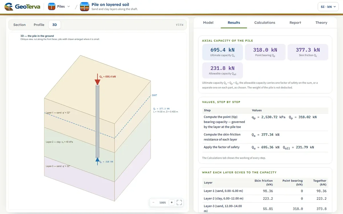
A 0.4 m circular pile, 14 m long, through sand over clay over sand — 6 m of sand at φ′ = 32°, 6 m of clay at cu = 40 kPa and a sand below it, with the water table at 3 m, K = 1.0, δ′ = 24°, α = 0.5 and a factor of safety of 3. This is the profile the module opens with.
The point — the tip is in the third layer, a sand
The shaft — layer by layer
so Qu = 702 kN and, at FS = 3, Qall = 234 kN. Press Analyze on the Model tab to see the same numbers with every step written out.
10ReferencesSources.
- Meyerhof, G.G. (1976). Bearing capacity and settlement of pile foundations. Journal of the Geotechnical Engineering Division, ASCE, 102(GT3), 197–228.
- Vesic, A.S. (1977). Design of Pile Foundations. NCHRP Synthesis of Highway Practice 42, Transportation Research Board.
- Terzaghi, K., Peck, R.B. and Mesri, G. (1996). Soil Mechanics in Engineering Practice, 3rd ed. Wiley — the α values of Table 2.
- Coyle, H.M. and Castello, R.R. (1981). New design correlations for piles in sand. Journal of the Geotechnical Engineering Division, ASCE, 107(GT7), 965–986.
- Vijayvergiya, V.N. and Focht, J.A. (1972). A new way to predict capacity of piles in clay. Offshore Technology Conference Paper 1718, Houston.
- O’Neill, M.W. and Reese, L.C. (1999). Drilled Shafts: Construction Procedures and Design Methods. FHWA-IF-99-025 — the drilled-shaft α of a bored pile.
- Reese, L.C. and O’Neill, M.W. (1989). Drilled Shafts: Construction Procedures and Design Methods. FHWA — the base expression of a drilled shaft in clay.
- Burland, J.B. (1973). Shaft friction of piles in clay — a simple fundamental approach. Ground Engineering, 6(3), 30–42.
- Mansur, C.I. and Hunter, A.H. (1970). Pile tests, Arkansas River project. Journal of the Soil Mechanics and Foundations Division, ASCE, 96(SM5), 1545–1582.
- Das, B.M. (2016). Principles of Foundation Engineering, 8th ed. Cengage Learning, which brings these methods together in the form this page follows.
From theory to your own design
Find the capacity of your own pile through layers in minutes
- The ultimate and the allowable capacity with the share of every layer
- Up to eight layers, each typed as sand or clay with its own method
- Diagrams of the shaft and the point resistance and a 3D view of the layers and the pile
- A clean calculation report, saved as a PDF. Online: nothing to install, no dongle, on a phone, a tablet or a PC