
On this page · 14 chapters
- 1What the pile carries
- 2Why clay is treated undrained
- 3Point bearing
- 4Meyerhof — the fixed nine
- 5Vesic — the stiffness enters
- 6Skin friction — three routes
- 7The α method
- 8The λ method
- 9The β method
- 10A bored pile: the drilled-shaft procedure
- 11The three routes compared
- 12Allowable capacity
- 13Worked example
- 14References
A pile in clay carries its load the same two ways a pile in sand does, but the clay against the shaft is never quite the clay the borehole sampled — which is why three different routes to the skin friction are in common use, and why this page spends most of its length on them.
 PDF
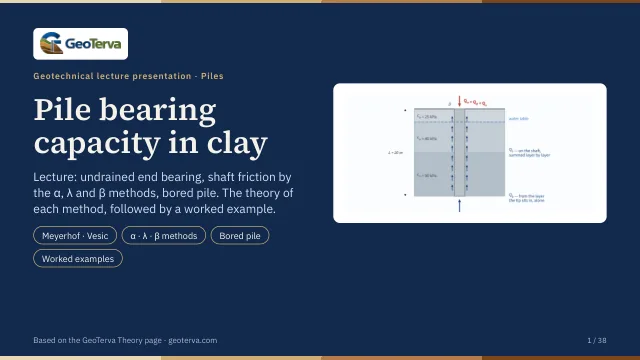
Lecture slides
Ready-made slides for lectures and self-study
The mechanism, the derivation, the equations and the figures of this page, in teaching order. Every slide links back to its chapter.
1What the pile carriesQᵤ = Qₚ + Qₛ and the allowable load.
A pile carries its load in two ways at once: the clay under the tip resists like a deep footing, and the clay along the shaft resists by adhesion. The ultimate capacity is the sum of the two, and the allowable capacity follows from a single factor of safety on that sum.
This module is for a single pile in clay, driven or bored, of constant cross section — square or circular. Up to eight clay layers may be described, each with its own undrained strength. Group action, negative skin friction from a consolidating layer, and settlement are separate subjects, each with a calculation of its own.
2Why clay is treated undrainedφ = 0, and where σ′ still enters.
In a saturated clay the load of a structure arrives far faster than the water can leave, so the clay is sheared without changing volume. In that state the strength is a single number — the undrained shear strength cu — and the friction angle is zero. This is the great difference from a pile in sand: the resistance no longer grows in proportion to the effective stress, so a pile in clay is not a pile in sand with another set of numbers.
Two of the routes below nevertheless need the effective vertical stress: the λ method uses its average over the embedded length, and the β method is built on it entirely, because it describes the clay long after driving, when it has drained. The water table therefore still matters — not to the point resistance and not to the α method, but to those two.
3Point bearingqₚ = N*c·cᵤ under the tip.
Clay (φ = 0)
In a saturated clay under undrained conditions the friction angle is zero, and the net ultimate point bearing capacity of the pile is a factor times the undrained cohesion of the clay below the tip:
The strength of the clay the shaft passed through on the way down plays no part here: it belongs to the shaft, not to the point. In a typical profile the point is also much the smaller of the two parts — for the worked pile below it is about one-ninth of the total.
4Meyerhof — the fixed nineN*c = 9, whatever the clay.
For piles in saturated clay under undrained conditions the net ultimate load is given, in Meyerhof’s form, by the classical factor of nine:
with cu the undrained cohesion of the soil below the tip of the pile. It takes no further input and does not depend on how deep the pile is, provided it is deep — a few diameters is enough.
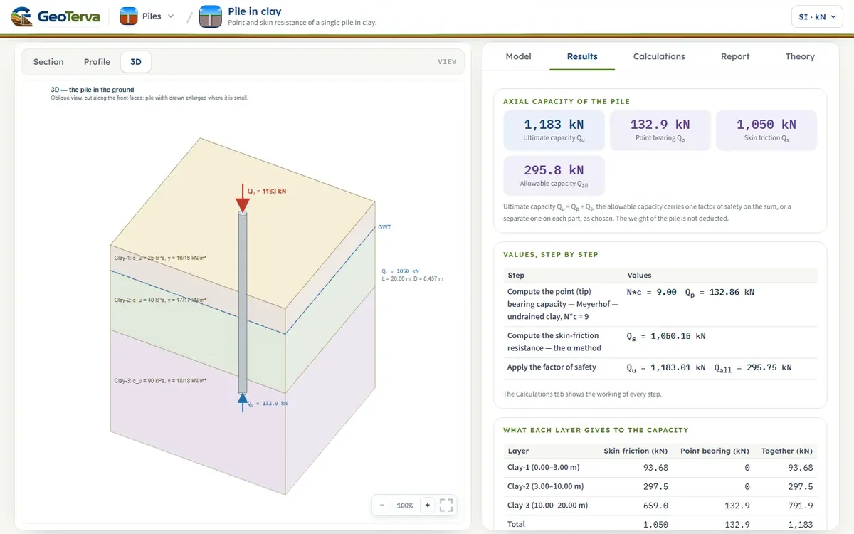
For the worked pile, with cu = 90 kPa at the tip, qp = 810 kPa and Qp = 132.9 kN.
5Vesic — the stiffness entersN*c from the rigidity index.
According to the expansion of cavity theory of Vesic (1977), the factor of the φ = 0 condition follows from the reduced rigidity index of the clay:
| Irr | N*c |
|---|---|
| 10 | 6.97 |
| 20 | 7.90 |
| 40 | 8.82 |
| 60 | 9.36 |
| 80 | 9.75 |
| 100 | 10.04 |
| 200 | 10.97 |
| 300 | 11.51 |
| 400 | 11.89 |
| 500 | 12.19 |
In a saturated clay sheared without a change of volume the average volumetric strain in the plastic zone is zero, so the reduction falls away and Irr = Ir; and for φ = 0 the rigidity index itself is
O’Neill and Reese (1999) relate Ir to the strength directly — Ir ≈ 50 at cu/pa = 0.24, 150 at 0.48 and 250 to 300 for cu/pa ≥ 0.96 — and those values are approximated by
which is the form this module uses, so the only number it needs for Vesic’s factor is the undrained strength at the tip. At cu = 90 kPa it gives Irr = 279.3 and N*c = 11.41, about a quarter more than the fixed nine.
6Skin friction — three routesWhere the capacity is really decided.
Estimating the frictional resistance of a pile in clay is almost as difficult as estimating it in sand: several of the variables that decide it cannot easily be quantified. Several methods are described in the literature; the three this module offers are the ones the source examines.
- the α method takes the friction from the undrained strength alone — total stress, short term;
- the λ method mixes the average effective stress with the average strength, one coefficient for the whole pile;
- the β method takes it from the effective stress and a remoulded friction angle — drained, long term.
The shaft is where the capacity of a pile in clay is decided: for the worked pile it is close to nine-tenths of the total. That is also where the uncertainty is.
7The α methodA fraction of the undrained strength.
The unit skin resistance in a clay is written as a fraction of the undrained strength, with an empirical adhesion factor α:
| cu/pa | α |
|---|---|
| ≤ 0.1 | 1.00 |
| 0.2 | 0.92 |
| 0.3 | 0.82 |
| 0.4 | 0.74 |
| 0.6 | 0.62 |
| 0.8 | 0.54 |
| 1.0 | 0.48 |
| 1.2 | 0.42 |
| 1.4 | 0.40 |
| 1.6 | 0.38 |
| 1.8 | 0.36 |
| 2.0 | 0.35 |
| 2.4 | 0.34 |
| 2.8 | 0.34 |
The values of α vary somewhat, because α is in truth a function of the vertical effective stress as well as of the undrained cohesion. The source lists the proposals that follow from that: Sladen (1992) writes α = C(σ̄′o/cu)0.45 with C ≈ 0.4 to 0.5 for bored piles and ≥ 0.5 for driven ones; the correlation of Randolph and Murphy (1987), taken into the API code, gives α = 0.5(cu/σ′o)−0.5 for cu/σ′o ≤ 1 and the same form with the exponent −0.25 above it; and the NGI-99 method of Karlsrud et al. (2005) brings the plasticity index in.
This module reads the interpolated table above. For the worked pile the three layers give α = 0.87, 0.74, 0.51, and Qs = 1050 kN.
8The λ methodOne average over the whole length.
The method of Vijayvergiya and Focht (1972) rests on the assumption that the soil displaced by driving the pile produces a passive lateral pressure at every depth, and that the average unit skin resistance follows from it:
where σ̄′o is the mean effective vertical stress over the whole embedded length and cu the mean undrained shear strength. The coefficient λ changes with the depth of penetration of the pile:
| L (m) | λ |
|---|---|
| 0 | 0.500 |
| 5 | 0.336 |
| 10 | 0.245 |
| 15 | 0.200 |
| 20 | 0.173 |
| 25 | 0.150 |
| 30 | 0.136 |
| 35 | 0.132 |
| 40 | 0.127 |
| 50 | 0.118 |
| 60 | 0.113 |
| 70 | 0.110 |
| 80 | 0.110 |
| 90 | 0.110 |
Care is needed with the two averages in a layered soil. The mean strength is weighted by the thickness of each layer — (cu(1)L1 + cu(2)L2 + …)/L — and the mean effective stress is the area of the effective-stress diagram divided by the length, σ̄′o = (A1 + A2 + A3 + …)/L:
For the worked pile σ̄′o = 98.85 kPa, c̄u = 62.75 kPa, λ = 0.173, fav = 38.81 kPa and Qs = 1114 kN — and the module computes both averages the way the figure shows.
9The β methodEffective stress and a remoulded skin.
The β method is the effective-stress approach of Burland, with the overconsolidation adjustment after Meyerhof. It leaves the undrained strength aside altogether and works from the vertical effective stress and the drained friction angle of the clay in its remoulded state (c′ = 0). At any depth,
with K the earth-pressure coefficient, taken conservatively at rest and raised for an overconsolidated clay by √OCR. The two combine into one expression, which at OCR = 1 reduces of itself to the normally consolidated form — there are not two rules:
Two things the module will not guess
φ′R and OCR are entered, not correlated. The source defines the remoulded drained friction angle but gives no relation to read it from, so nothing can be filled in from the ground: each φ′R box simply opens at 30° and each OCR box at 1. These stand until they are replaced with the values that belong to the clays in hand — φ′R from a remoulded or residual shear test where there is one.
What the profile looks like
Because f follows σ′(z), the unit friction grows with depth inside a layer and steps where β changes at a boundary — it is not constant over a layer as it is in the α method. The layer average f̄ = βσ̄′ is what gives that layer’s share of Qs, since βσ̄′ΔL is the integral of βσ′(z) over it; the module draws the real f(z) and reports the average beside it.
The mean is the true integral over the layer, not the average of its two ends — a distinction that matters as soon as the water table crosses a layer, where the two differ by more than ten per cent.
For the worked pile, with φ′R = 30° and the lowest layer at OCR = 2, Qs = 1058 kN.
10A bored pile: the drilled-shaft procedureα* = 0 over two lengths, and a base of its own.
A bored pile — a drilled shaft — is not a driven pile with smaller numbers. The hole is drilled and the concrete cast in it: nothing is displaced, the clay at the wall of the hole softens as it takes up water, debris collects under the base, and the base needs a larger settlement to develop its resistance. The source gives a procedure of its own for it, and the module follows that procedure on both halves of the capacity when the pile is bored.
The shaft
The adhesion factor is no longer read from the curve fitted to driven piles. The drilled-shaft rule of O’Neill and Reese gives α = 0.55 up to cu/pa = 1.5, falling to 0.45 at 2.5 — and, as important, it sets α to zero over two lengths of the shaft:
The top 1.5 m is the ground most disturbed by the work and the most likely to shrink away from the shaft; the bottom diameter is the length over which the base is already mobilising the soil. The module applies both as a window on the integration: the layer thicknesses are never altered, so depth and effective stress stay as the profile describes them, and only the length that carries friction changes.
The base
The base is worked from the clay beneath it rather than from a bearing-capacity factor alone: the resistance grows with how deep the shaft is relative to its own base, and is then held by two ceilings.
cub is the mean undrained strength over the 2Db below the base — not the value at the tip alone, which is why the module asks for the ground to be described that far down and says so in the report when it has to take the deepest layer as continuing. Where that zone spans more than one layer, cub is their thickness-weighted mean.
A wide base would need an unacceptable settlement to reach qp, so for Db greater than 1.91 m the value is reduced:
with c1 = 2.78×10⁻⁴ + 8.26×10⁻⁵(L/Db) ≤ 5.9×10⁻⁴ and c2 = 0.065√cub between 0.5 and 1.5, Db in millimetres.
11The three routes comparedHow far apart do they land?
On the worked pile the three shaft routes land within a few per cent of one another. That is worth looking at squarely: they agree here, but they do not agree in principle, and the agreement is a property of this profile rather than a general result.
Change the profile and they separate: a very long pile pulls the λ method down through its coefficient, a heavily overconsolidated clay pulls the β method up through √OCR, and a soft normally consolidated clay pushes the α method up towards the full strength of the soil. The honest reading of a spread like this is that the shaft resistance of a pile in clay is known to perhaps a fifth by calculation alone, which is why a load test is worth what it costs on a large job.
12Allowable capacityOne factor of safety on the sum.
The ultimate capacity is the sum of the two parts, and the allowable capacity carries one factor of safety over the whole of it:
A factor of 2.5 to 4 is usual for a single pile, the higher end where the ground is known only from a few boreholes, where the clay is stiff and fissured, or where no load test is planned. Enter the working load and the module checks it against Qall.
13Worked exampleThe 20 m pile in three clay layers.
A 457 mm pipe pile, 20 m long, driven through three clay layers — 3 m of cu = 25 kPa, 7 m of 40 kPa and 10 m of 90 kPa, with the water table at 3 m. The module opens with this pile.
The point
The shaft, by the α method
With Meyerhof’s point and the α shaft, Qu = 1183 kN and, at FS = 4, Qall = 296 kN. Every number on this page can be reproduced by pressing Analyze on the Model tab.
14ReferencesSources.
- Das, B.M. (2016). Principles of Foundation Engineering, 8th ed. Cengage Learning; this page follows it.
- Terzaghi, K., Peck, R.B. and Mesri, G. (1996). Soil Mechanics in Engineering Practice, 3rd ed. Wiley — the α values of Table 2.
- O’Neill, M.W. and Reese, L.C. (1999). Drilled Shafts: Construction Procedures and Design Methods. FHWA-IF-99-025 — the drilled-shaft α and the rigidity index of a clay.
- Reese, L.C. and O’Neill, M.W. (1989). Drilled Shafts: Construction Procedures and Design Methods. FHWA — the base expression of a drilled shaft in clay.
- Burland, J.B. (1973). Shaft friction of piles in clay — a simple fundamental approach. Ground Engineering, 6(3), 30–42.
- Meyerhof, G.G. (1976). Bearing capacity and settlement of pile foundations. Journal of the Geotechnical Engineering Division, ASCE, 102(GT3), 197–228 — the √OCR adjustment of the β method.
- Vijayvergiya, V.N. and Focht, J.A. (1972). A new way to predict the capacity of piles in clay. Offshore Technology Conference, Paper 1718, Houston.
- Vesic, A.S. (1977). Design of Pile Foundations. NCHRP Synthesis of Highway Practice 42, Transportation Research Board.
From theory to your own design
Find the capacity of your own pile in clay in minutes
- The point and the skin resistance, the ultimate and the allowable capacity
- The α, λ or β factor with its numbers, layer by layer
- The resistance diagrams along the pile
- A clean calculation report, saved as a PDF. Online: nothing to install, no dongle, on a phone, a tablet or a PC