
On this page · 16 chapters
- 1Scope
- 2The cone data
- 3Unit weight and stresses
- 4Soil behaviour type index
- 5Screening of the readings
- 6Boulanger & Idriss (2014) — normalisation
- 7Boulanger & Idriss (2014) — resistance
- 8Robertson & Wride (1998) — NCEER
- 9Cyclic stress ratio
- 10Factor of safety
- 11Zones and thickness
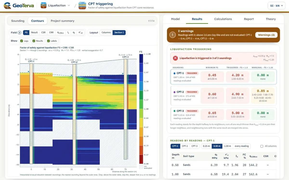
- 12Colour-band section
- 13Reading the two procedures side by side
- 14A worked reading
- 15What the module does not do
- 16References
The module checks whether liquefaction is triggered at each reading of a cone penetration test (CPT) below the groundwater table, with one of two CPT-based procedures: Boulanger & Idriss (2014) and Robertson & Wride (1998) as recommended by the NCEER workshops. For every sounding it gives the factor of safety against depth, the depth ranges where liquefaction is triggered and a project summary of all soundings; between soundings it draws colour bands over a section.
 PDF
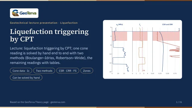
Lecture slides
Ready-made slides for lectures and self-study
The mechanism, the derivation, the equations and the figures of this page, in teaching order. Every slide links back to its chapter.
1Scope
The cone gives a nearly continuous record (a reading every 1 to 5 cm), so there is no layer table to enter: the soil type, the unit weight and the fines content are all estimated from the cone data. A boring next to the sounding, with laboratory fines contents, is the way to check them.
Consequences of liquefaction — settlement, lateral spreading, loss of bearing capacity — are outside this version.
2The cone data
qc is the measured tip resistance, fs the sleeve friction, u2 the pore pressure measured behind the cone tip and a the net area ratio of the cone (0.65 to 0.85; 0.80 is a common value). The correction matters in soft clays and silts, where u2 is far above the hydrostatic value, and is small in sands. When no u2 is recorded, qt = qc is used and the module says so.
Columns are read in MPa (qc) and kPa (fs, u2); the unit of a column may be written in its heading when the data is imported or pasted — MPa, kPa, kN/m², kg/cm², bar, tsf, psi, atm. A unit that is written like a unit but is not one of these stops the import: it is never replaced by the default. A column of corrected cone resistance qt is turned back into qc with the net area ratio and u2; a friction ratio column is turned into fs = Rf·qt.
Pa is one atmosphere, 101.325 kPa, in both procedures (the NCEER text rounds it to 100 kPa; the difference is below 1 % of qc1N). In the unit systems of the page qc, fs and u2 are shown in one unit — kg/cm² or tsf — except in SI · kN, where the convention of the cone is kept (qc in MPa, fs and u2 in kPa).
3Unit weight and stresses
The unit weight of every reading is estimated from the CPT (Rf in %, kept between 1.5 γw and 2.5 γw) and integrated from the surface; or two constant values are used, γ above and γsat below the groundwater level. The pore pressure is hydrostatic from the groundwater level.
Two groundwater depths are kept. The cone resistance reflects the stresses that acted at the time of the test, so its normalisation (CN, Ic) uses the groundwater depth of the test. The earthquake acts on the design groundwater level — often the high seasonal level — and CSR and Kσ use that. When the design depth is left blank it is the depth of the test.
4Soil behaviour type index
The exponent n runs from 0.5 in sands to 1.0 in clays and is found by the iteration of Robertson & Wride (1998): with n = 1.0, an Ic above 2.6 means a clay and n stays 1.0; otherwise n = 0.5 is tried, and when Ic is then still above 2.6 the soil is in between and n = 0.75 is used. The formula is used as published; only F is kept at 0.1 % or more, so that a sleeve reading of zero does not give the logarithm of zero.
| Ic | Zone | Soil behaviour type |
|---|---|---|
| < 1.31 | 7 | gravelly sand to dense sand |
| 1.31 – 2.05 | 6 | sands: clean sand to silty sand |
| 2.05 – 2.60 | 5 | sand mixtures: silty sand to sandy silt |
| 2.60 – 2.95 | 4 | silt mixtures: clayey silt to silty clay |
| 2.95 – 3.60 | 3 | clays: silty clay to clay |
| > 3.60 | 2 | organic soils: peats |
The soil log of the drawings is this classification; a run thinner than hmin joins its longer neighbour.
5Screening of the readings
A reading is evaluated when it lies below the design groundwater level, not deeper than zmax (20 m by default; the stress reduction relationships are not verified deeper) and in soil that behaves like sand. Soil is clay-like when Ic is above Ic,lim (2.6 by default). Clay-like soil can soften under cyclic loading but does not liquefy in the sense used here, so it is left to a cyclic-softening check.
The cut-off between sand-like and clay-like behaviour is not sharp. The NCEER workshops recommend sampling every soil with Ic of 2.4 or more; the Boulanger & Idriss procedure suggests repeating the analysis with Ic,lim = 2.4, 2.6 and 2.8 to see how much it matters. The module lists the evaluated readings with Ic between 2.4 and the limit among its warnings.
A reading whose net cone resistance qt − σv is not positive has no soil behaviour index and is not evaluated. Readings that are not evaluated stay in every table, with the reason.
The input is checked before the analysis, and a value outside the range the procedures were built for is refused, not corrected: a magnitude outside 4 to 9.5, a peak ground acceleration above 2 g, unit weights outside 10 to 30 kN/m³ (a value in t/m³ typed into a box in kN/m³ is caught here), a depth of more than 150 m, a cone resistance of more than 150 MPa, a sounding without sleeve friction, two soundings of one name. A negative groundwater depth is allowed — it is water standing above the ground surface.
6Boulanger & Idriss (2014) — normalisation
The exponent depends on the result, so CN is found by iteration; qc1Ncs is kept between 21 and 254 in m. σ′v is the effective stress at the time of the test. CFC is the fitting parameter of the correlation between Ic and fines content (0 is the general correlation; ±0.29 is one standard deviation of it). The correlation scatters widely, so a site-specific CFC from laboratory fines contents of boreholes next to the soundings is the better value; it should be fitted per geological stratum.
7Boulanger & Idriss (2014) — resistance
The curve is the deterministic one of the report (the 16th percentile of the case-history data — constant 2.80). qc1Ncs above 211 is taken at 211, where Cσ reaches its limit; such soil is very dense and the factor of safety is large. σ′v in Kσ is the effective stress of the design groundwater level.
8Robertson & Wride (1998) — NCEER
The exponent n is the one found with Ic. The last rule is the one of the flow chart of the paper: a soil with Ic between 1.64 and 2.36 and a friction ratio below 0.5 % is a clean, non-plastic sand whose Ic is raised by the cone resistance alone, and it gets no fines adjustment. The chart of the clean-sand curve ends at (qc1N)cs = 160, where the workshops call the soil too dense to liquefy: the module continues the same cubic to 250 (CRR7.5 = 1.5) and flags the reading, so that a factor of safety is always given. MSF is the revised relationship, which the workshops recommend as the lower bound for magnitudes below 7.5 and for use above 7.5. Kσ is the equation of Hynes & Olsen with the exponent f an input — 0.7 to 0.8 for relative densities of 40 to 60 %, 0.6 to 0.7 for 60 to 80 % — and 1.0 where σ′v does not exceed Pa. The correction of the workshops for sloping ground (Kα) and for age is not applied.
9Cyclic stress ratio
σv and σ′v are the stresses of the design groundwater level, z the depth in metres, amax the peak ground acceleration at the surface in units of g, Mw the moment magnitude. The magnitude and overburden corrections are applied to the resistance, not to the demand.
10Factor of safety
| Result | Condition |
|---|---|
| Triggered | FS < 1.0 |
| Marginal | 1.0 ≤ FS < FSreq |
| OK | FS ≥ FSreq |
FSreq is an input: set it from the project specification or the code that applies. The factor of safety of a CPT is a continuous record that scatters with the soil variability and the noise of the instrument; thin layers are not resolved by the cone (its zone of influence is several cone diameters), so a single low reading is not a layer.
11Zones and thickness
Each reading stands for the depth halfway to the reading above and halfway to the reading below, but for not more than a quarter of a metre (or three quarters of the usual reading interval, where that is larger) on either side: a gap in the record is not extrapolated into results — it stays a not evaluated run, written “no readings”, and a warning lists it. At the design groundwater level and at zmax the interval stops. Consecutive readings with the same result form a run. A run of one result thinner than hmin (0.10 m by default, the resolution of the cone) takes the result of its longer neighbour, and neighbouring runs with the same result are merged into zones; not evaluated runs are never absorbed. The triggered and marginal thicknesses are the sums of the zones. hmin = 0 lists every run as it is.
The minimum factor of safety is the lowest value of any single evaluated reading and is shown with its depth; for a CPT it is sensitive to noise, and the thickness is the steadier figure.
12Colour-band section
The Contours view paints a field over the soundings: each sounding gives the field against depth from its readings; with a section the field is interpolated linearly between neighbouring soundings at equal elevation and the nearest sounding is used beyond the outer ones; without a section every sounding is drawn as its own colour column. Grey means not evaluated: at or above the water table, clay-like soil, deeper than zmax or no readings (the top of a pre-drilled sounding, a gap in the record). The fields are FS, the result class, CSR, CRR, qc1Ncs, Ic, qt and σ′v0.
13Reading the two procedures side by side
Each procedure is a package: its stress reduction, its normalisation, its clean-sand adjustment, its magnitude and overburden factors and its resistance curve were derived together from a case-history database, and the sources of the two procedures ask that the components of one are not mixed with those of the other. The module keeps them apart: choosing the method changes all of them at once.
Differences between the two come mainly from the fines adjustment — Kc multiplies and the Boulanger & Idriss adjustment adds — and from the stress reduction at depth. A project that is sensitive to the choice is a project for site-specific sampling and testing.
14A worked reading
CPT-1 of the example project at z = 4.00 m: qc = 4.956 MPa, fs = 46.2 kPa, u2 = 21.6 kPa, groundwater at 1.80 m, amax = 0.35 g, Mw = 7.5. The two procedures are two complete packages; their numbers are not meant to be mixed.
| Quantity | Boulanger & Idriss (2014) | Robertson & Wride (1998) |
|---|---|---|
| Corrected cone resistance qt (kPa) | 4960 | 4960 |
| Unit weight γ (kN/m³) | 18.01 | 18.01 |
| σ′v at the test (kPa) | 52.05 | 52.05 |
| Soil behaviour index Ic | 2.031 | 2.031 |
| Stress exponent n of Ic | 0.50 | 0.50 |
| Fines content FC (%) | 25.5 | not used |
| CN · CQ | 1.374 | 1.395 |
| qc1N | 67.25 | 68.30 |
| Fines adjustment Δqc1N · Kc | 42.74 | 1.343 |
| qc1Ncs · (qc1N)cs | 109.99 | 91.73 |
| rd | 0.9718 | 0.9694 |
| CSR | 0.3127 | 0.3120 |
| CRR at M 7.5 and 1 atm | 0.1520 | 0.1518 |
| MSF | 1.000 | 1.000 |
| Kσ | 1.077 | 1.000 |
| CRR | 0.1636 | 0.1517 |
| Factor of safety FS | 0.52 | 0.49 |
15What the module does not do
The cone resistance is used as measured: no thin-layer correction of stiff layers between soft ones and no transition-zone removal where the cone passes from one soil to another (the Ic of a transition from clay to sand reads as silt). Where such zones are suspected the analysis can be repeated on edited data. No correction for age, cementation, static shear stress (Kα) or sloping ground is made, the procedures are deterministic (no probability of liquefaction), and nothing is said about cyclic softening of the clay-like soils, about the consequences of liquefaction or about the shear-wave velocity.
The procedures were derived for Holocene, uncemented, silica sands and silty sands, level or gently sloping ground, depths of 1 to 12 m, earthquakes of magnitude 6 to 8 and Ic below about 2.6. Beyond that — gravels, carbonate sands, depths of more than 15 to 20 m, M above 8 — the results are an indication to be checked by a specialist.
16References
- Boulanger, R.W., Idriss, I.M. (2014). CPT and SPT based liquefaction triggering procedures. Report UCD/CGM-14/01, University of California, Davis.
- Robertson, P.K., Wride, C.E. (1998). Evaluating cyclic liquefaction potential using the cone penetration test. Canadian Geotechnical Journal, 35(3), 442–459.
- Youd, T.L., Idriss, I.M. et al. (2001). Liquefaction resistance of soils: summary report from the 1996 NCEER and 1998 NCEER/NSF workshops. J. Geotech. Geoenviron. Eng., 127(10), 817–833.
- Robertson, P.K. (1990). Soil classification using the cone penetration test. Canadian Geotechnical Journal, 27(1), 151–158.
- Robertson, P.K., Cabal, K.L. (2010). Estimating soil unit weight from CPT. Proc. 2nd International Symposium on Cone Penetration Testing, Huntington Beach.
- Idriss, I.M. (1999). An update to the Seed–Idriss simplified procedure for evaluating liquefaction potential. Proc. TRB Workshop, FHWA-RD-99-165.
- Liao, S.S.C., Whitman, R.V. (1986). Overburden correction factors for SPT in sand. J. Geotech. Eng., ASCE, 112(3).
- Hynes, M.E., Olsen, R.S. (1999). Influence of confining stress on liquefaction resistance. Proc. International Workshop on the Physics and Mechanics of Soil Liquefaction, Balkema.
- Idriss, I.M., Boulanger, R.W. (2008). Soil liquefaction during earthquakes. EERI Monograph MNO-12.
From theory to your own design
Check liquefaction at your own site in minutes
- The soil log, the normalised cone resistance, the cyclic ratios and the factor of safety, reading by reading
- Triggered and marginal zones, and sections between soundings
- A project summary and a Word report
- A clean calculation report, saved as a PDF. Online: nothing to install, no dongle, on a phone, a tablet or a PC